Free sample chapter from FRM Level I: Risk Models.
Chapter 1: Measures of Financial Risk
Chapter 1: Measures of Financial Risk
Foundations of Risk Management gave Ravensmoor Financial Group a capital number for every risk it runs, each one a loss that would be exceeded only once in a thousand years. Financial Markets and Products I and II priced the instruments behind those numbers. This course asks the question the earlier courses took for granted: where does a risk number come from?
The answer, which every chapter of this course repeats in a different setting, is that a risk number is a percentile of a distribution, and somebody chose the distribution. This chapter makes the point on the simplest position the group owns. The $800 million Core Equity Fund has a volatility of 18% a year — that number has not changed since Foundations. But a volatility is not a distribution. Two return distributions with exactly the same 18% volatility give the fund a one-day 99.9% value at risk of $28.03 million and $46.01 million.
The chapter starts where risk measurement started, with standard deviation in the mean-variance framework, and shows why one number stopped being enough. It defines value at risk, finds the questions VaR cannot answer, and introduces the measure that answers them — expected shortfall. It then sets out the four properties any sensible risk measure should have, and shows with two small loans that VaR fails one of them.
- $28.03M vs $46.01M Fund one-day 99.9% VaR (normal against fat-tailed returns, both with 18% volatility)
- $30.54M vs $62.13M Fund one-day 99.9% expected shortfall (the fat tail doubles it)
- $0 + $0 < $10M Two loans, 95% VaR (each alone has none; together they do)
Learning Objectives
Learning objectives
- Explain risk as standard deviation in the mean-variance framework and locate the efficient frontier and tangency portfolio
- Contrast the normal distribution with the fat-tailed, skewed returns of real equities
- Define value at risk, compute it for a normal position at any confidence and horizon, and explain its limitations
- Compute expected shortfall and contrast it with VaR
- State and interpret the four properties of a coherent risk measure
- Show why VaR is not coherent, explain why expected shortfall is, and describe spectral risk measures
1.1 Risk and Return in the Mean-Variance Framework
The first quantitative definition of investment risk, Harry Markowitz's in 1952, was the standard deviation of return. An investor cares about two things — the expected return of a portfolio and its standard deviation — and prefers more of the first and less of the second.
For a portfolio with weight in asset 1 and in asset 2, the two quantities are
The expected return is a weighted average. The standard deviation is not: unless the correlation is exactly 1, the portfolio's standard deviation is less than the weighted average of the two, and that difference is the benefit of diversification.
The efficient frontier
Ravensmoor's asset-allocation committee chooses between two asset classes:
| Expected return | Volatility | |
|---|---|---|
| Equities | 8.0% | 18.0% |
| Government bonds | 3.8% | 4.5% |
| Correlation | 0.10 |
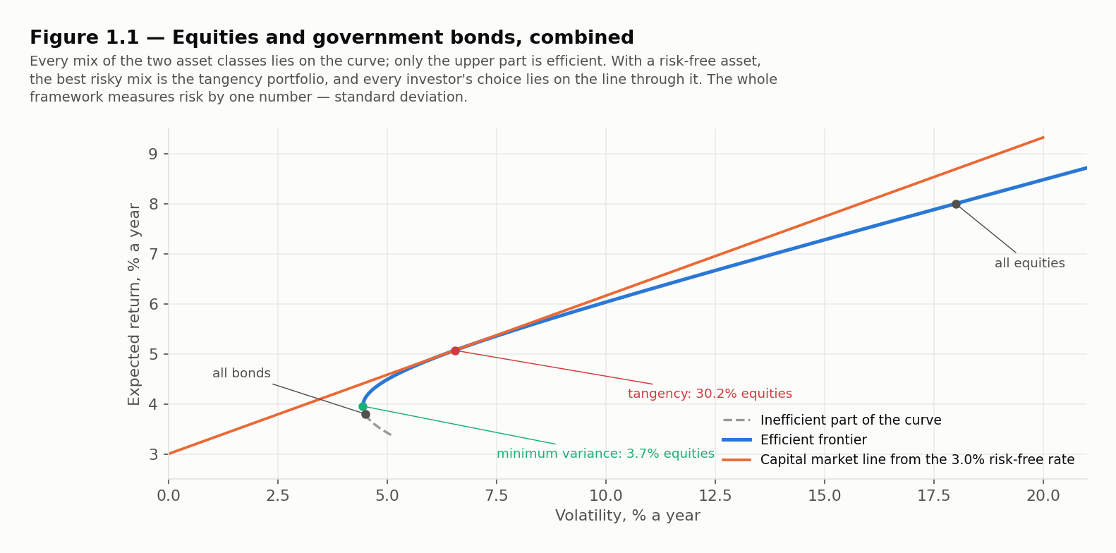
Every mix of the two traces out a curve in the plane of volatility and expected return. The point on it with the smallest volatility is the minimum-variance portfolio. Points below it on the curve are inefficient — another mix has the same volatility and a higher return. The part above it is the efficient frontier: for each level of risk, the highest return available.
Efficient frontier The set of portfolios that offer the highest expected return for a given standard deviation — equivalently, the lowest standard deviation for a given expected return. No rational mean-variance investor holds a portfolio below it.
Worked Problem — The Minimum-Variance Mix
Problem. Using the table above, find the weight in equities that minimises the portfolio's volatility, and that portfolio's expected return and volatility.
Solution. The portfolio variance is a quadratic in — plotted against it is a U-shaped curve — and its lowest point is where the curve is flat, its slope zero. Solving for the at that point gives
with equities as asset 1. The covariance is , so
The minimum-variance portfolio holds 3.70% equities. Its expected return is , and its volatility is 4.45% — slightly less than the 4.5% of bonds alone, even though it adds an asset four times as volatile. Low correlation pays.
BA II Plus keystrokes: The Minimum-Variance Weight — Equity vol 18%; bond vol 4.5%; correlation 0.10
| Keys | Display | Note |
|---|---|---|
| 0.1 × 0.18 × 0.045 = STO 1 | → 0.00081 | covariance, stored in memory 1 |
| 0.045 x² - RCL 1 = STO 2 | → 0.001215 | numerator, stored in memory 2 |
| RCL 1 × 2 = STO 3 | → 0.00162 | twice the covariance, computed first because chain mode keys left to right |
| 0.18 x² + 0.045 x² - RCL 3 = STO 4 | → 0.032805 | the denominator |
| RCL 2 ÷ RCL 4 = | → 0.037037 | 3.70% in equities |
In chain mode, keying 0.18 [x²] [+] 0.045 [x²] [-] 2 [×] [RCL] 1 would compute (0.0324 + 0.002025 − 2) × 0.00081, not the denominator, which is why the doubled covariance is computed first and recalled.
The tangency portfolio and the capital market line
Add a risk-free asset yielding 3.0%. Any investor can now hold a mix of the risk-free asset and one risky portfolio, and those mixes lie on a straight line from the risk-free rate through the risky portfolio. The steepest such line touches the frontier at the tangency portfolio — the risky mix with the highest Sharpe ratio, . That line is the capital market line, and every mean-variance investor holds a point on it: a cautious one lends at the risk-free rate, an aggressive one borrows.
For two risky assets, the tangency weight has a closed form in their excess returns over the risk-free rate, and , and their covariance :
Worked Problem — The Tangency Portfolio
Problem. Using the table above and a risk-free rate of 3.0%, find the weight in equities of the tangency portfolio, and that portfolio's expected return, volatility and Sharpe ratio.
Solution. The excess returns are for equities and for bonds, and the covariance is 0.00081 as before. The numerator is
and the denominator is
so : the tangency portfolio holds 30.23% equities. Its expected return is . Its variance is
so its volatility is , and its Sharpe ratio is , or 0.3161 with the weight unrounded — against for equities alone and for bonds alone. No other mix of the two earns more excess return per unit of volatility.
BA II Plus keystrokes: The Tangency Weight — Excess returns 5.0% and 0.8%; equity vol 18%; bond vol 4.5%; correlation 0.10
| Keys | Display | Note |
|---|---|---|
| 0.1 × 0.18 × 0.045 = STO 1 | → 0.00081 | covariance, stored in memory 1 |
| 0.05 × 0.045 x² = STO 2 | → 0.00010125 | equity excess return times bond variance |
| 0.008 × RCL 1 = STO 3 | → 0.00000648 | bond excess return times covariance |
| RCL 2 - RCL 3 = STO 4 | → 0.00009477 | the numerator |
| 0.008 × 0.18 x² = STO 5 | → 0.0002592 | bond excess return times equity variance |
| 0.058 × RCL 1 = STO 6 | → 0.00004698 | sum of excess returns times covariance |
| RCL 2 + RCL 5 - RCL 6 = | → 0.00031347 | the denominator; chain mode is safe for a run of + and − |
| 1/x × RCL 4 = | → 0.302326 | 30.23% in equities |
Validation: the minimum-variance and tangency portfolios
from math import sqrt

mu_e, sd_e, mu_b, sd_b, rho, rf = 0.08, 0.18, 0.038, 0.045, 0.10, 0.03
cov = rho * sd_e * sd_b

def portfolio(w):
    mean = w * mu_e + (1 - w) * mu_b
    sd = sqrt(w ** 2 * sd_e ** 2 + (1 - w) ** 2 * sd_b ** 2 + 2 * w * (1 - w) * cov)
    return mean, sd

w_min = (sd_b ** 2 - cov) / (sd_e ** 2 + sd_b ** 2 - 2 * cov)
ex_e, ex_b = mu_e - rf, mu_b - rf
w_tan = (ex_e * sd_b ** 2 - ex_b * cov) / (ex_e * sd_b ** 2 + ex_b * sd_e ** 2 - (ex_e + ex_b) * cov)
for name, w in (("minimum variance", w_min), ("tangency", w_tan)):
    m, s = portfolio(w)
    print(f"{name:<16} equities {w:.2%}   return {m:.2%}   volatility {s:.2%}   Sharpe {(m - rf) / s:.4f}")
# Output:
# minimum variance equities 3.70%   return 3.96%   volatility 4.45%   Sharpe 0.2147
# tangency         equities 30.23%   return 5.07%   volatility 6.55%   Sharpe 0.3161
What the framework assumes
Standard deviation is a complete description of risk only if the distribution of returns is fully described by its mean and standard deviation — which is true of the normal distribution — or if investors care about nothing else. Neither holds well for real assets. Standard deviation also treats a large gain as just as "risky" as a large loss, which no risk manager believes. The rest of this chapter is about what replaced it.
1.2 How Real Returns Depart From the Normal
The normal distribution is attractive: it is described by two numbers, sums of normal variables are normal, and its percentiles are tabulated. Daily returns on equities and most risky assets, though, differ from it in three consistent ways.
- Fat tails (excess kurtosis). Very large moves, in both directions, happen far more often than a normal distribution with the same standard deviation allows. The kurtosis of daily equity returns is typically well above the normal's 3.
- Negative skew. The largest moves are more often falls than rises: markets tend to drift up and crash down. A normal distribution is symmetric.
- Volatility clustering. Large moves follow large moves. Volatility is not constant; it rises in bad periods and stays high for a while. Chapter 3 models this directly.
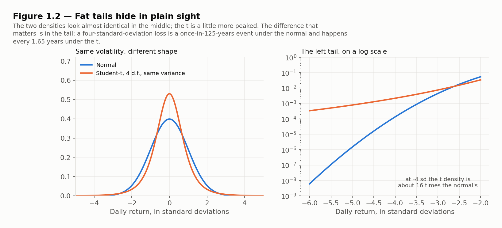
There is also a fourth, quieter difference: daily returns tend to be more peaked than the normal near zero. With the same total variance, the distribution puts more probability in the very centre and in the far tails, and less in the shoulders between.
Same volatility, different tail
The cleanest way to see what fat tails do is to hold the volatility fixed and change only the shape. This course uses a Student-t distribution with 4 degrees of freedom, rescaled so that its standard deviation equals that of the normal. A t with degrees of freedom has variance , so the scaling factor that gives unit variance is
The t is symmetric, so it captures fat tails but not skew. That is a simplification, and not a conservative one: real equity returns put extra mass in the left tail, which a symmetric t spreads equally over both, so it can understate the left tail it is meant to measure.
Worked Problem — How Often Is a Four-Sigma Day?
Problem. Daily returns have a standard deviation . With 252 trading days a year, how often should a loss larger than occur if returns are normal, and how often if they follow the rescaled t with 4 degrees of freedom?
Solution. Under the normal, : once every 31,574 trading days, or once in 125 years.
Under the rescaled t, a loss of is a loss of in the units of a standard t with 4 degrees of freedom, and : once every 1.65 years.
Neither tail probability is a calculator calculation: the normal value is read from the far tail of a z-table and the t value from statistical software or a t table, and the validation block below reproduces both. The same move is 76 times more likely. A risk manager who calibrated to the normal would be surprised by a "once-in-a-century" loss roughly every twenty months — which is close to the experience of equity markets.
Validation: how often large losses arrive, normal against fat-tailed
from math import sqrt
from scipy.stats import norm, t

nu = 4
scale = sqrt((nu - 2) / nu)          # rescales a t(4) variable to unit variance
for k in (3, 4, 5):
    p_normal = norm.cdf(-k)
    p_t = t.cdf(-k / scale, nu)
    print(f"loss beyond {k} sd: normal once in {1 / p_normal / 252:>9,.1f} years   "
          f"t(4) once in {1 / p_t / 252:5.2f} years")
# Output:
# loss beyond 3 sd: normal once in       2.9 years   t(4) once in  0.60 years
# loss beyond 4 sd: normal once in     125.3 years   t(4) once in  1.65 years
# loss beyond 5 sd: normal once in  13,843.5 years   t(4) once in  3.76 years
Volatility Is Not a Distribution
A five-sigma day is a once-in-14,000-years event under the normal and a once-in-four-years event under the t — with the same standard deviation. Volatility tells you the scale of typical moves. It tells you nothing about how often the extreme ones come, and the extreme ones are what risk management is for.
1.3 Value at Risk
Standard deviation answers "how much do returns typically vary?" A risk manager, a board or a regulator wants an answer to a different question: how much could we lose? Value at risk was built to answer it in one number.
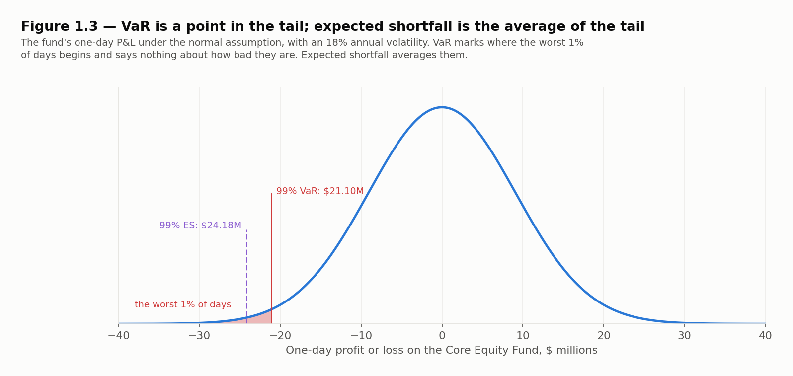
Value at risk (VaR) The loss over a stated time horizon that will not be exceeded with a stated probability, the confidence level. A one-day 99% VaR of $21 million means that on 99% of days the loss should be no more than $21 million — equivalently, that the loss exceeds $21 million on 1% of days.
A VaR number therefore has two parameters that must always be stated with it:
- the confidence level , typically 95%, 99% or 99.9%;
- the time horizon , typically one day or ten days for trading books and one year for credit and capital.
Formally, if is the loss over the horizon, VaR at confidence is the -quantile of the loss distribution: the smallest for which . Because VaR is stated as a loss, it is reported as a positive number.
VaR when returns are normal
If returns over the horizon are normal with mean and standard deviation , and the position is worth , the loss is normal too, and
where is the standard normal percentile: 1.6449 for 95%, 2.3263 for 99% and 3.0902 for 99.9%. Over a short horizon such as one day, the expected return is tiny compared with the standard deviation and is normally set to zero, which gives the simplest and most quoted form, .
Scaling across horizons — the square-root-of-time rule
Daily volatility and annual volatility are linked by the number of trading days. If daily returns are independent and identically distributed, variances add across days, so standard deviations grow with the square root of time:
With 252 trading days, an annual volatility of 18% is a daily volatility of . The rule is used everywhere — Basel's ten-day market-risk VaR was for years computed as one-day VaR times — but it rests on two assumptions that real returns break:
- Independence. If returns are autocorrelated, the rule is wrong. Positive autocorrelation (trends) makes multi-day losses larger than the rule says; negative autocorrelation (mean reversion), smaller.
- Identical distribution with zero mean. Volatility clustering means tomorrow's volatility depends on today's, so the ten-day distribution is not a scaled-up one-day distribution. And over long horizons the mean is no longer negligible: it grows with while the standard deviation grows only with .
Worked Problem — A One-Day and a Ten-Day VaR
Problem. A $50 million equity position has a daily volatility of 1.2%. Compute its one-day VaR at 95% and 99%, and its ten-day 99% VaR using the square-root rule. Assume a zero mean.
Solution. The daily standard deviation in dollars is 50,000,000 × 0.012 = $600,000.
- One-day 95% VaR: 600,000 × 1.6449 = $986,940
- One-day 99% VaR: 600,000 × 2.3263 = $1,395,780
- Ten-day 99% VaR: 1,395,780 × = $4,413,844
With the percentiles to more decimal places the three figures are $986,912, $1,395,809 and $4,413,935; the differences are rounding in , not in the method.
BA II Plus keystrokes: Ten-Day 99% VaR — Position $50M; daily vol 1.2%; z(99%) = 2.3263
| Keys | Display | Note |
|---|---|---|
| 50000000 × 0.012 × 2.3263 = | → 1,395,780 | one-day 99% VaR |
| × 10 √x = | → 4,413,844 | ten-day 99% VaR; [√x] acts on the 10 at once |
What VaR assumes, and what it does not
VaR is a definition, not a model. To compute it, you need the distribution of the position's loss over the horizon — and every choice about that distribution changes the answer:
- The shape of the distribution. Normal, fat-tailed, or the empirical distribution of past returns (Chapter 2's historical simulation).
- The volatility. A long-run average, a recent estimate, or the market's implied volatility (Chapter 3).
- The holding period. The horizon should be the time it would take to close or hedge the position. A liquid equity book can be cut in a day; a book of illiquid loans cannot, and a one-day VaR on it is meaningless.
- The portfolio is fixed over the horizon. VaR asks what happens to today's positions, not to whatever the traders hold next week.
1.4 VaR on the Core Equity Fund, Normal and Fat-Tailed
The Core Equity Fund is worth $800 million with an annual volatility of 18%. Its daily standard deviation is
That is $9.07 million. Under the normal, the one-day 99% VaR is $21.10 million, and the ten-day 99% VaR by the square-root rule is $66.73 million.
BA II Plus keystrokes: The Fund's One-Day 99% VaR — Fund $800M; annual vol 18%; 252 days; z(99%) = 2.3263
| Keys | Display | Note |
|---|---|---|
| 252 √x | → 15.874508 | square root of the trading days, keyed first |
| 1/x × 0.18 × 800000000 = | → 9,071,147 | one-day standard deviation in dollars |
| × 2.3263 = | → 21,102,210 | one-day 99% VaR, $21.10 million |
Over one day the mean barely matters. If the fund is expected to return 8% a year, the one-day expected gain is 800 × 0.08 / 252 = $0.25 million, which lowers the VaR from $21.10 million to $20.85 million. Over a year it matters a great deal: the one-year 99% VaR is $334.99 million with a zero mean and $270.99 million after subtracting the $64 million expected gain.
The same fund, fat-tailed
Now keep everything — the $800 million, the 18% volatility — and change only the distribution, to the rescaled t with 4 degrees of freedom. The one-day VaR becomes the daily standard deviation times the t's percentile times 0.7071. The t(4) percentiles, read from a t table, are 2.1318, 3.7469 and 7.1732 at 95%, 99% and 99.9%, against the normal's 1.6449, 2.3263 and 3.0902. So at 99.9% the fat-tailed VaR is 9,071,147 × 7.1732 × 0.7071 = $46.01 million; at 99% it is 9,071,147 × 3.7469 × 0.7071 = $24.03 million; and at 95% it is 9,071,147 × 2.1318 × 0.7071 = $13.67 million.
| Confidence | Normal VaR | Fat-tailed VaR | Fat-tailed ÷ normal |
|---|---|---|---|
| 95% | $14.92M | $13.67M | 0.92 |
| 99% | $21.10M | $24.03M | 1.14 |
| 99.9% | $28.03M | $46.01M | 1.64 |
Two things stand out. First, at 99.9% the fat-tailed VaR is 64% higher. Second, at 95% it is lower. That is the more peaked shape of §1.2 at work: with the same variance, the t puts more probability right at the centre and in the far tail, so less of it falls in the moderate losses that a 95% VaR measures. A fat-tailed distribution is not "riskier everywhere". It moves risk into the far tail, which is exactly where a 95% VaR does not look.
The confidence level is a choice too
A risk manager who wanted the fat tail to look harmless could report a 95% VaR, and it would show the fund as less risky than the normal model does. The confidence level should be set by what the number is for — capital at 99.9%, a trading limit at 99% — and never by the result it gives.
1.5 The Limitations of VaR
VaR became the industry's standard risk measure in the 1990s, through J.P. Morgan's RiskMetrics and then the Basel market-risk rules. Its appeal is real: one number, in currency, comparable across desks and asset classes, and easy to explain to a board. Its limitations are just as real.
- It says nothing about the size of losses beyond it. A 99% VaR of $21 million tells you that 1% of days are worse than $21 million. Whether those days lose $22 million or $200 million, VaR does not say.
- It can be gamed. Because VaR ignores everything past its percentile, a trader can lower it by taking on risk that sits just beyond the percentile — for example, by writing deep out-of-the-money options that lose rarely but heavily.
- It is only as good as its distribution. As §1.4 showed, the normal and fat-tailed VaRs of one fund differ by 64% at 99.9%. Past data are a poor guide to future tails, and a VaR estimated from a calm period understates the risk that arrives in a crisis.
- It is not subadditive. The VaR of a combined portfolio can exceed the sum of the VaRs of its parts, which means that VaR can penalise diversification. §1.8 shows how.
Worked Problem — A Book That VaR Cannot See
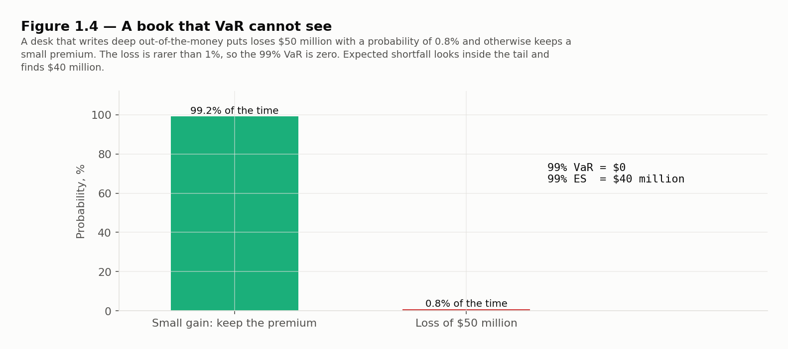
Problem. A trading desk writes deep out-of-the-money index puts. On any given day it keeps a small premium, except that with probability 0.8% the market falls far enough that it loses $50 million. Compute the desk's 99% one-day VaR and 99.5% one-day VaR, ignoring the premium.
Solution. The probability of a loss above zero is 0.8%. At 99% confidence, VaR is the smallest loss exceeded with probability at most 1%. A loss above $0 has probability 0.8%, which is less than 1%, so the 99% VaR is $0.
At 99.5% the tail is 0.5%, smaller than the 0.8% chance of losing $50 million, so the 99.5% VaR is $50 million.
A risk limit set on the 99% VaR would let this desk run the position without limit. Raising the confidence level a little reveals it, but a slightly rarer loss would hide it again: any loss rarer than one minus the confidence level is invisible to VaR.
1.6 Expected Shortfall
The natural repair for limitation 1 is to ask the question VaR refuses to answer: if we are in the tail, how bad is it on average?
Expected shortfall (ES) The expected loss over the horizon, given that the loss is in the worst of outcomes. Also called conditional VaR (CVaR), expected tail loss or tail conditional expectation. For a continuous distribution, it is the expected loss conditional on the loss exceeding VaR.
For a continuous loss distribution,
Expected shortfall is always at least as large as the VaR at the same confidence level, because it averages losses that are all at least VaR.
Expected shortfall for a normal position
When the loss is normal with zero mean and standard deviation , ES has a closed form:
where is the standard normal density (not the cumulative probability) at the percentile :
At 99%, , so the ES multiplier is , against 2.3263 for VaR: ES is 15% above VaR. At 97.5%, and the multiplier is — almost exactly the 99% VaR multiplier. That near-equality is why the Basel Committee, when it replaced 99% VaR with expected shortfall for market-risk capital, chose a 97.5% confidence level: under the normal the capital number barely changes, while under a fat tail it rises.
Worked Problem — The Fund's 99% Expected Shortfall
Problem. Compute the Core Equity Fund's one-day 99% expected shortfall under the normal distribution.
Solution. The density at is
or 0.026652 with the percentile carried to full precision (2.326348). Using that value, the ES is
The 99% ES is $24.18 million, against a 99% VaR of $21.10 million. On the worst 1% of days the fund loses $24.18 million on average.
BA II Plus keystrokes: Normal Expected Shortfall — Daily standard deviation $9,071,147; z(99%) = 2.3263
| Keys | Display | Note |
|---|---|---|
| 2 × 2nd π = √x 1/x STO 1 | → 0.398942 | 1 over the square root of 2 pi, stored first |
| 2.3263 x² ÷ 2 = +/- 2nd eˣ | → 0.066814 | e to the minus z squared over two |
| × RCL 1 = | → 0.026655 | the density (0.026652 with z to more places) |
| ÷ 0.01 × 9071147 = | → 24,179,243 | 99% ES, $24.18 million |
The constant is stored first because the square-root key acts on whatever is displayed: keyed at the end of a chain, it would take the root of the whole running result rather than of 2π.
The keystrokes end at $24,179,243 rather than the Worked Problem's $24,176,421 because they carry to four places, 2.3263, where the Worked Problem used the full 2.326348. The $2,822 gap is rounding in , and both figures round to $24.18 million.
The fund's ES, normal and fat-tailed
The t distribution's expected shortfall also has a closed form. Nothing on the exam requires it; it is shown here for reference only, so that the fat-tailed column below can be reproduced by hand. With the t percentile and the standard t density,
At 99%, , so and . The multiplier is , and 9,071,147 × 3.6916 is $33.49 million. The same steps at 95% (, , multiplier 2.2648) and at 99.9% (, , multiplier 6.8491) give $20.54 million and $62.13 million.
| Confidence | Normal ES | Fat-tailed ES | Fat-tailed ÷ normal |
|---|---|---|---|
| 95% | $18.71M | $20.54M | 1.10 |
| 99% | $24.18M | $33.49M | 1.39 |
| 99.9% | $30.54M | $62.13M | 2.03 |
Notice that at 95%, where the fat-tailed VaR was lower than the normal one, the fat-tailed ES is higher. ES looks past the percentile and into the tail, so it sees the fat tail at every confidence level. At 99.9% it doubles.
Validation: the fund's VaR and ES under both distributions
from math import sqrt
from scipy.stats import norm, t

fund, vol, nu = 800e6, 0.18, 4
sd_day = fund * vol / sqrt(252)
scale = sqrt((nu - 2) / nu)

for c in (0.95, 0.99, 0.999):
    z = norm.ppf(c)
    q = t.ppf(c, nu)
    var_n, es_n = sd_day * z, sd_day * norm.pdf(z) / (1 - c)
    var_t = sd_day * q * scale
    es_t = sd_day * scale * t.pdf(q, nu) / (1 - c) * (nu + q * q) / (nu - 1)
    print(f"{c:.1%}  normal VaR {var_n / 1e6:6.2f}M  ES {es_n / 1e6:6.2f}M   "
          f"t(4) VaR {var_t / 1e6:6.2f}M  ES {es_t / 1e6:6.2f}M")
print(f"10-day 99% VaR, normal: {sd_day * norm.ppf(0.99) * sqrt(10) / 1e6:.2f}M")
# Output:
# 95.0%  normal VaR  14.92M  ES  18.71M   t(4) VaR  13.67M  ES  20.54M
# 99.0%  normal VaR  21.10M  ES  24.18M   t(4) VaR  24.03M  ES  33.49M
# 99.9%  normal VaR  28.03M  ES  30.54M   t(4) VaR  46.01M  ES  62.13M
# 10-day 99% VaR, normal: 66.73M
Expected shortfall for a discrete distribution
For a discrete distribution, ES is the probability-weighted average of the worst of outcomes, taking a fraction of an outcome when the tail boundary falls inside it. The put writer of §1.5 loses $50 million with probability 0.8%. Its 99% tail is 1% wide: 0.8% of it is the $50 million loss and the remaining 0.2% is a loss of zero. So
The 99% ES is $40 million for a desk whose 99% VaR is zero. ES cannot be gamed by hiding losses just past the percentile, because it counts them.
VaR and ES compared
| Value at risk | Expected shortfall | |
|---|---|---|
| Question it answers | How bad is the threshold of the tail? | How bad is the tail on average? |
| Sees losses beyond the percentile | No | Yes |
| Subadditive (§1.8) | Not always | Always |
| Backtesting | Simple: count days the loss exceeds it | Harder: it is an average of rare events |
| Estimation | Needs one percentile | Needs the whole tail, so noisier |
| Regulatory use | Basel market risk until the FRTB | Basel market risk since the FRTB, at 97.5% |
The last two rows are VaR's remaining advantages. VaR can be checked by counting exceptions — Chapter 2 shows how — while ES depends on the few observations deep in the tail, so it is estimated less precisely and checked less easily.
1.7 Coherent Risk Measures
VaR and ES are two candidates. How should anyone decide which is better, or whether some third measure is better than both? In 1999 Artzner, Delbaen, Eber and Heath answered by asking what properties any sensible risk measure should have. A risk measure assigns a number — the capital needed — to each portfolio's future value. They proposed four properties, and called a measure that has all four coherent.
Coherent risk measure A risk measure that satisfies monotonicity, translation invariance, positive homogeneity and subadditivity.
1. Monotonicity. If portfolio has a lower value than portfolio in every state of the world, then is at least as risky: . A portfolio that always does worse cannot need less capital.
2. Translation invariance. Adding a riskless amount of cash to a portfolio reduces its risk measure by exactly :
This is what lets a risk measure be read as capital. If a portfolio's risk measure is $21 million, adding $21 million of cash brings it to zero: the cash covers the loss.
3. Positive homogeneity. Scaling a portfolio by a positive factor scales its risk by the same factor:
Doubling every position doubles the capital required. This assumes the position can be scaled without changing its character — a strong assumption for a large position in an illiquid market, where selling twice as much costs more than twice as much.
4. Subadditivity. The risk of a combined portfolio is no greater than the sum of the risks of its parts:
This is the mathematical form of diversification. Merging two portfolios should never create extra risk. If it could, a firm could lower its measured risk by splitting itself into pieces, and a regulator could not add up the capital of a firm's desks and know the total was enough.
Why Subadditivity Is the Property That Matters
Monotonicity, translation invariance and positive homogeneity are satisfied by VaR and ES alike. They are not automatic: standard deviation fails two of them, since adding cash leaves it unchanged rather than lowering it, and a portfolio that always does worse can have the smaller standard deviation. Between VaR and ES, though, subadditivity is the property that separates them. It is also the one that makes risk management workable: if the firm-wide risk measure is subadditive, the sum of the desks' limits is a ceiling on the firm's risk.
1.8 Why VaR Is Not Coherent
When returns are normal — or, more generally, elliptical — VaR is subadditive, because it is then a fixed multiple of standard deviation, and standard deviation is subadditive. The failure comes from discrete, lumpy losses, exactly the kind a loan book produces.
Worked Problem — Two Loans
Problem. A bank holds two independent loans of $10 million each. Each defaults over the year with probability 4%, and a default loses the whole $10 million. Compute the one-year 95% VaR of each loan on its own and of the two together. Then compute the 95% expected shortfall in both cases.
Solution — VaR. Each loan alone loses $10 million with probability 4%. Because 4% is less than the 5% tail, the 95% VaR of each loan is $0, and the sum of the two standalone VaRs is $0.
For the pair, with independent defaults:
| Outcome | Probability | Loss |
|---|---|---|
| No default | $0 | |
| One default | $10M | |
| Both default | $20M |
The probability of losing more than $0 is , more than 5%, so the VaR is at least $10 million. The probability of losing more than $10 million is 0.16%, less than 5%. So the 95% VaR of the pair is $10 million:
VaR fails subadditivity. Combining two loans appears to create $10 million of risk.
Solution — expected shortfall. For one loan, the 5% tail consists of the 4% default ($10 million) and 1% of the no-default outcome ($0):
Each loan's 95% ES is $8 million, and the two sum to $16 million. For the pair, the 5% tail is the 0.16% double default at $20 million plus 4.84% of the single-default outcome at $10 million:
The pair's ES is $10.32 million, less than the $16 million sum. Expected shortfall registers the diversification that VaR penalised.
BA II Plus keystrokes: The Pair's 95% Expected Shortfall — PD 4% each, independent; loss $10M per default; 5% tail
| Keys | Display | Note |
|---|---|---|
| 0.04 x² STO 1 | → 0.0016 | probability both default |
| 0.05 - RCL 1 = STO 2 | → 0.0484 | the slice of the one-default outcome inside the tail |
| RCL 1 × 20 = STO 3 | → 0.032 | double-default contribution |
| RCL 2 × 10 + RCL 3 = | → 0.516 | chain mode: 0.484 plus 0.032 |
| ÷ 0.05 = | → 10.32 | 95% ES of the pair, $10.32 million |
Validation: two loans, VaR against expected shortfall
# Two independent $10M loans, each defaulting with probability 4% and losing everything
p, size, c = 0.04, 10.0, 0.95

p_both = p * p
p_one = 2 * p * (1 - p)
print(f"P(no default) {(1 - p) ** 2:.4f}   P(one) {p_one:.4f}   P(both) {p_both:.4f}")

# VaR: the smallest loss L with P(loss > L) <= 5%
var_single = 0.0 if p <= 1 - c else size
var_pair = 0.0 if p_one + p_both <= 1 - c else (size if p_both <= 1 - c else 2 * size)
print(f"95% VaR: each loan {var_single:.2f}, sum {2 * var_single:.2f}, both together {var_pair:.2f}")

# ES: the average loss in the worst 5% of outcomes
es_single = size * p / (1 - c)
es_pair = (p_both * 2 * size + ((1 - c) - p_both) * size) / (1 - c)
print(f"95% ES:  each loan {es_single:.2f}, sum {2 * es_single:.2f}, both together {es_pair:.2f}")
# Output:
# P(no default) 0.9216   P(one) 0.0768   P(both) 0.0016
# 95% VaR: each loan 0.00, sum 0.00, both together 10.00
# 95% ES:  each loan 8.00, sum 16.00, both together 10.32
What the example generalises to
The loans are small, but the mechanism is general. A VaR treats any loss rarer than its tail as if it did not exist. Each loan's default, at 4%, is rarer than the 5% tail; combine two loans and the chance of some default, 7.84%, is not. Diversification spread the loss into more frequent, smaller pieces, and VaR saw them for the first time.
Expected shortfall is coherent for every distribution: it satisfies all four properties. Why it is subadditive can be seen without algebra. ES at confidence is the largest average loss over any set of outcomes with total probability : the worst of outcomes give the highest average, and any other set of the same size gives less. Now take the worst of outcomes for the combined portfolio . Its ES is 's average loss over those outcomes plus 's average loss over the same outcomes. Those outcomes need not be the worst ones for alone, so 's average over them is at most ; likewise 's is at most . Hence . VaR has no such argument, because it is not an average over a set of outcomes but a single cut-off, and the cut-off of a sum can sit above the sum of the cut-offs, as the two loans showed.
That subadditivity, together with its sensitivity to the size of tail losses, is why the Basel Committee moved market-risk capital from VaR to ES. VaR keeps its place where losses are close to normal and where its ease of backtesting matters.
1.9 Spectral Risk Measures and Risk Aversion
VaR and ES can both be written as weighted averages of the loss quantiles. Let be the loss at percentile (so is the 99% VaR), and let be a weight on each percentile. A spectral risk measure is
The integral sign here only means a weighted average: multiply each quantile by its weight and add them up across all percentiles, exactly as a weighted average of a list of numbers does.
The two measures of this chapter are special cases:
- VaR at confidence puts all of its weight on one percentile, , and none anywhere else.
- ES at confidence puts zero weight on percentiles below and an equal weight of on every percentile above it.
A spectral risk measure is coherent if and only if its weights are non-negative, sum to one, and never decrease as rises — that is, if a worse outcome never gets less weight than a better one. This is how the weights should reflect risk aversion: a risk-averse investor cares more about worse outcomes. ES meets the condition, with weights flat across the tail. VaR does not: its weight drops from everything to nothing just past , so the outcomes worse than VaR get less weight than VaR itself.
A common choice is the exponential spectrum, , which rises smoothly towards the worst outcomes; the parameter is the degree of risk aversion. The larger , the more the measure concentrates on the far tail.
Validation: an exponential spectral measure on the fund
from math import sqrt, exp
import numpy as np
from scipy.stats import norm, t

sd_day, nu = 800e6 * 0.18 / sqrt(252), 4
scale = sqrt((nu - 2) / nu)
p = (np.arange(200_000) + 0.5) / 200_000            # midpoints of the probability scale


def spectral(k, quantile):
    weight = k * np.exp(-k * (1 - p)) / (1 - exp(-k))   # rises with p: worse outcomes weigh more
    return np.mean(weight * quantile)


normal_q = sd_day * norm.ppf(p)
t_q = sd_day * scale * t.ppf(p, nu)
for k in (25, 100):
    print(f"risk aversion k = {k:>3}:  normal {spectral(k, normal_q) / 1e6:6.2f}M   "
          f"t(4) {spectral(k, t_q) / 1e6:6.2f}M")
# Output:
# risk aversion k =  25:  normal  17.73M   t(4)  19.57M
# risk aversion k = 100:  normal  22.73M   t(4)  30.28M
For a mildly risk-averse holder (), the fat tail adds 10% to the measure; for a strongly risk-averse one (), it adds 33%. The more a measure cares about the worst outcomes, the more the choice of distribution drives it.
1.10 Putting It All Together: What the Fund Can Lose Tomorrow
Ravensmoor's board asks the chief risk officer a simple question: how much could the Core Equity Fund lose tomorrow? Every input the CRO needs has been fixed since Foundations: $800 million, an 18% volatility, a one-day horizon. The answer still depends on two choices this chapter has made explicit.
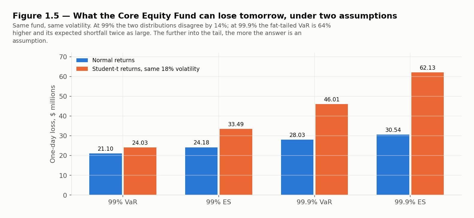
| Measure | Normal | Fat-tailed | Difference |
|---|---|---|---|
| 99% VaR | $21.10M | $24.03M | +14% |
| 99% ES | $24.18M | $33.49M | +39% |
| 99.9% VaR | $28.03M | $46.01M | +64% |
| 99.9% ES | $30.54M | $62.13M | +103% |
The choice of distribution. Volatility pins down the typical day, not the bad ones. With an identical 18% volatility, a fat tail adds 14% to the 99% VaR and doubles the 99.9% ES. The data the CRO has — a few years of daily returns — contains only a handful of days beyond the 99th percentile and perhaps none beyond the 99.9th, so the shape of the far tail is largely an assumption.
The choice of measure. VaR says where the tail begins; ES says how bad it is. At 95%, VaR would report that the fat-tailed fund is safer. ES would not. And of the two tail measures, only ES is guaranteed to reward the diversification that the mean-variance framework of §1.1 was built to capture.
A responsible answer to the board is therefore not one number but a short table and a sentence: on one day in a hundred we expect to lose more than about $21 to $24 million, and on those days about $24 to $33 million on average, depending on how fat the tail is. The width of each range is the honest part of the answer.
The Course's Thesis, in One Fund
The $800 million and the 18% never changed. The answers ranged from $13.67 million to $62.13 million. Every number in that range is a percentile, or an average of percentiles, of a distribution somebody chose. The rest of this course changes one choice at a time — the estimation method, the volatility estimate, the rating philosophy, the correlation, the severity tail, the scenario — and measures what each one moves.
Chapter Summary
What You Learned in Chapter 1
- The mean-variance framework measures risk by standard deviation. For equities (8.0%, 18%) and bonds (3.8%, 4.5%) with correlation 0.10, the minimum-variance portfolio holds 3.70% equities with a 4.45% volatility, and the tangency portfolio holds 30.23% with a Sharpe ratio of 0.3161. The efficient frontier is the part of the curve above the minimum-variance point.
- Real returns depart from the normal: fat tails, negative skew, volatility clustering and a sharper peak. With the same volatility, a four-sigma loss is a once-in-125-years event under the normal and a once-in-1.65-years event under a t with 4 degrees of freedom.
- VaR is the loss not exceeded with probability over horizon . Under the normal, , with = 1.6449, 2.3263 and 3.0902 at 95%, 99% and 99.9%. The square-root-of-time rule scales VaR by and requires independent, identically distributed returns.
- The fund's one-day 99% VaR is $21.10 million under the normal ($66.73 million over ten days); its 99.9% VaR is $28.03 million normal and $46.01 million fat-tailed. At 95% the fat-tailed VaR is lower.
- VaR's limitations: it ignores losses beyond the percentile, can be gamed (the put writer's 99% VaR is $0), depends on the assumed distribution and is not subadditive.
- Expected shortfall is the average loss in the worst of outcomes; under the normal, . The fund's 99% ES is $24.18 million; its 99.9% ES doubles from $30.54 million to $62.13 million under the fat tail. The 97.5% ES is close to the 99% VaR under the normal.
- A coherent risk measure satisfies monotonicity, translation invariance, positive homogeneity and subadditivity.
- VaR is not coherent: two independent $10 million loans with 4% default probability each have a 95% VaR of $0, but together $10 million. Their ES is $8 million each and $10.32 million combined — subadditive.
- Spectral risk measures weight the loss quantiles; they are coherent when the weights never fall as outcomes worsen. ES uses flat tail weights, VaR a single spike.
What's Next
This chapter took the distribution as given — normal or t — and computed from it. Chapter 2 asks how VaR and ES are computed in practice, when the distribution is unknown and the portfolio contains more than a single equity fund: by historical simulation from past returns, by the delta-normal method for linear positions and options, and by Monte Carlo simulation. Applied to one Ravensmoor portfolio, the three methods give three different answers, and each difference has a cause that can be named.
Concept Checks
-
A trading desk reports a one-day 99% VaR of $5 million. What does this tell you?
- The desk's average loss on its worst 1% of days is $5 million
- The desk cannot lose more than $5 million on any single trading day, whatever happens
- The desk's one-day loss should exceed $5 million on about 1% of days
- The desk loses $5 million on 99% of days and more on the rest
-
Which limitation of VaR does the put-writing desk illustrate, with its 0.8% chance of a $50 million loss and a 99% VaR of zero?
- VaR ignores the size of any loss rarer than one minus the confidence level
- VaR cannot be computed for positions whose returns are not normally distributed
- VaR requires the square-root-of-time rule, which fails for options
- VaR overstates the risk of option positions because it ignores the premium received
-
A risk-free asset is added to a frontier of equities and bonds. Under the mean-variance framework, how do the holdings of a cautious and an aggressive investor differ?
- The cautious one holds the minimum-variance mix and the aggressive one holds only equities
- Both hold the minimum-variance mix, and the aggressive one borrows to buy more of it
- The cautious one holds only bonds and the aggressive one holds only equities, the curve's two ends
- Both hold the tangency portfolio, the cautious one adding lending and the aggressive one borrowing
-
Portfolio X is worth less than portfolio Y in every possible state of the world. Which property of a coherent risk measure requires that X be assigned at least as much risk as Y?
- Positive homogeneity
- Monotonicity
- Subadditivity
- Translation invariance
-
A portfolio's risk measure is $12 million. The firm adds $12 million of cash to the portfolio. Under translation invariance, what is the new risk measure?
- $12 million, because cash carries no risk and changes nothing
- $24 million, because adding the cash doubles the size of the portfolio being measured
- $6 million, because the cash covers half of the potential loss
- Zero, because the cash exactly offsets the capital the risk measure requires
-
Why is subadditivity regarded as the most important of the four coherence properties for a bank?
- It ensures the risk measure rises in line with the size of each position
- It ensures the measure can be expressed in units of currency and read as capital
- It ensures merging portfolios never increases measured risk, so desk limits add up to a ceiling
- It ensures the measure always gives more weight to worse outcomes than to better ones
-
Which statement about VaR and expected shortfall is correct?
- Expected shortfall is coherent for every distribution, while VaR can fail subadditivity
- VaR and expected shortfall are both coherent, because each measures losses in the tail
- VaR is coherent for every distribution, while expected shortfall fails monotonicity
- Neither is coherent, because both fail translation invariance whenever losses are discrete
-
What assumption does the square-root-of-time rule for scaling VaR across horizons require?
- Returns are fat-tailed, so that the tail grows faster than the variance
- Returns are independent and identically distributed from one day to the next
- Returns are positively autocorrelated, so that losses build on one another from day to day
- The portfolio is rebalanced to constant weights at the end of each day
-
How do the daily returns of equities typically differ from a normal distribution with the same mean and standard deviation?
- They have thinner tails and positive skew, so large rises are more common than equally large falls
- They are identical to the normal at the daily horizon and diverge only over months
- They have uniform tails, with extreme gains and losses equally likely at every size
- They have fatter tails and negative skew, with large falls more frequent than large rises
-
Under what condition is a spectral risk measure coherent?
- Its weights fall as outcomes worsen, so that it is not dominated by rare extremes
- Its weights are concentrated on a single percentile, as VaR's are
- Its weights are non-negative, sum to one and never fall as outcomes worsen
- Its weights are equal across every percentile from the best outcome to the worst
Exam-Style Practice
Ten standalone questions in the style of the FRM Level I exam. Allow 24 minutes — the exam's pace of 2.4 minutes a question.
Chapter 1 — Measures of Financial Risk
-
A $50 million equity position has a daily return volatility of 1.2%. Assuming normally distributed returns with a mean of zero, what is its one-day 99% VaR? The standard normal percentiles are 1.644854 at 95%, 2.326348 at 99% and 3.090232 at 99.9%.
- $986,912
- $1,395,809
- $4,413,935
- $1,854,139
-
A $20 million portfolio has normally distributed daily returns with a mean of zero and a volatility of 1.5%. The standard normal density at the 97.5% percentile, z = 1.96, is 0.058445. What is the portfolio's one-day 97.5% expected shortfall?
- $588,000
- $799,564
- $697,904
- $701,340
-
A portfolio has a one-day 99% VaR of $2.4 million. Using the square-root-of-time rule, what is its ten-day 99% VaR?
- $7.59 million
- $0.76 million
- $5.37 million
- $24.00 million
-
A risk manager doubles the size of every position in a portfolio, keeping the same proportions. Under a coherent risk measure, what happens to the measured risk?
- It rises by less than double, because the larger portfolio is more diversified
- It is unchanged, because the portfolio's weights are the same as before
- It doubles, because positive homogeneity requires the measure to scale with the position
- It rises by the square root of two, because risk scales with standard deviation
-
A bank holds two independent bonds of $5 million each. Each defaults over the year with probability 3%, losing its whole value. What is the one-year 95% VaR of the two bonds held together, and what is the sum of their standalone 95% VaRs?
- $5 million together; $0 for the sum
- $0 together; $0 for the sum
- $10 million together; $10 million for the sum
- $5 million together; $10 million for the sum
-
A position's one-day loss is $0 with probability 98.5%, $8 million with probability 1.0% and $20 million with probability 0.5%. What is its one-day 99% expected shortfall?
- $8 million
- $20 million
- $12 million
- $14 million
-
A $200 million portfolio has normally distributed annual returns with an expected return of 9% and a volatility of 20%. What is its one-year 95% VaR, taking account of the expected return? The standard normal percentiles are 1.644854 at 95% and 2.326348 at 99%.
- $65.79 million
- $47.79 million
- $83.79 million
- $75.05 million
-
An analyst replaces a normal distribution for a fund's daily returns with a fat-tailed Student-t distribution rescaled to the same volatility. Which of the following statements about the effect of this change is correct?
- VaR rises by the same proportion at every confidence level, because the volatility is unchanged
- VaR falls at every confidence level, because the t distribution is more peaked at the centre
- The 99.9% VaR rises, while the 95% VaR may fall as the shoulders of the distribution thin
- Expected shortfall is unchanged, because it depends only on the mean and volatility
-
Two assets have volatilities of 20% and 10% and a correlation of zero. What weight in the 20%-volatility asset gives the minimum-variance portfolio?
- 33.3%
- 20.0%
- 80.0%
- 50.0%
-
Why is VaR not a coherent risk measure?
- It can assign less risk to a portfolio that always performs worse than another
- Adding cash to a portfolio does not reduce its VaR by the amount added
- Scaling a position up does not scale its VaR by the same factor
- The VaR of a combined portfolio can exceed the sum of the VaRs of its parts