Free sample chapter from FRM Level I: Quantitative Analysis.
Chapter 1: Probability, Random Variables and Distributions
Chapter 1: Probability, Random Variables and Distributions
Quantitative Analysis is 20% of the FRM Level I exam, and almost every question in it is an estimate of something defined in this chapter. A regression coefficient is an estimate of a conditional expectation. A value-at-risk number is a quantile. A volatility is the square root of a second moment. A backtest is a hypothesis test about a probability. If the objects themselves are vague, everything built on them is vague too, and the vagueness is invisible — the arithmetic still produces a number.
So this chapter builds the objects. It does it on two pieces of Ravensmoor Financial Group, the institution this series follows.
The first is the bank's obligor default screen: a model that flags names it expects to default. It is 90% accurate in both directions, and the credit committee treats a flag as bad news. By §1.4 you will have shown that a flag is right 15.52% of the time, and that nothing is wrong with the model.
The second is Ravensmoor Asset Management's Core Equity Fund — $800 million, a reported 11.00% return against a benchmark's 9.20%, and a volatility of 18.00%. Those are the numbers the fund's own fact sheet quotes. This chapter turns them into a distribution; the rest of the course asks whether the distribution supports what the fact sheet claims.
- 15.52% Chance a flagged obligor actually defaults (from a screen that is 90% accurate both ways)
- 5.1962% The fund's monthly volatility (18.00% annual, scaled by the square root of 12)
- 7.4815 Kurtosis of two normal regimes mixed (neither component has any excess kurtosis at all)
Learning Objectives
Learning objectives
- Describe an event and an event space, and distinguish independent events from mutually exclusive ones
- Show, with an example, how two events can be dependent until a third is known and independent once it is
- Add up a probability mass function over the outcomes that make up an event
- Define and calculate a conditional probability, and differentiate conditional from unconditional probability
- Explain and apply Bayes' rule, and read what it says about a screening test
- Distinguish a probability mass function from a probability density function, and both from a cumulative distribution function
- Use expectation to compute a distribution's mean, variance, skewness and kurtosis, and say what each one measures
- Invert a cumulative distribution to read off quantiles, and say when the median and interquartile range describe data better than the mean and standard deviation
- Predict how rescaling and shifting a variable changes each of its summary statistics, and which ones it leaves alone
- Illustrate the key properties and applications of the eleven distributions the curriculum names
- Build a distribution from a calm regime and a stressed one, and show why the blend has fatter tails than either part
1.1 Events, Event Spaces and the Two Words People Confuse
Probability starts with a list of everything that could happen.
Sample space and event space The sample space is the set of all possible outcomes of an experiment. An event is any subset of it — a collection of outcomes you care about. The event space is the set of all events to which a probability can be assigned.
For one of Ravensmoor's obligors over one year the sample space is small: the borrower defaults, or it does not. For the Core Equity Fund's monthly return the sample space is the whole real line, and an event is an interval — "the fund loses more than 10%" is the event .
Three rules govern the assignment, and every later result is a consequence of them: a probability is never negative, the whole sample space has probability one, and the probability of a union of mutually exclusive events is the sum of their probabilities.
Mutually exclusive is not independent
These two are the most confused pair in the area, and the exam trades on it.
Mutually Exclusive and Independent Are Nearly Opposites
Mutually exclusive events cannot both happen: . Knowing that occurred tells you definitely did not, so mutually exclusive events are maximally dependent.
Independent events satisfy . Knowing that occurred tells you nothing at all about .
Two events with non-zero probability cannot be both. If they were mutually exclusive then , but independence would require .
"Obligor 1 defaults" and "obligor 2 defaults" are not mutually exclusive — both can happen, and in a recession both are likelier to. "The fund returns between 2% and 3% this month" and "the fund returns between 5% and 6% this month" are mutually exclusive, because a month has one return.
Unions, complements and the addition rule
Two consequences of the three rules do most of the everyday work. The complement rule, , turns "at least one" questions into "none" questions. The addition rule handles events that can overlap:
The subtraction removes the double count: outcomes in both and were added once with and again with . For mutually exclusive events the overlap is zero and the rule collapses to plain addition — the third axiom.
The event space is easy to picture for two obligors. The sample space has four outcomes, , where means the first defaults and the second does not. The event space holds every subset of those four — events, from the empty set to the whole space — and "at least one default" is the three-outcome event , the complement of .
Worked Problem — Speculative Grade or Default
Problem. Using the grade-by-default table in §1.2 below — 30.00% of obligors are speculative grade, 2.00% default, and 1.60% are both — what is the probability that a randomly chosen obligor is speculative grade or defaults? And what is the probability that two independent obligors, each defaulting with probability 2.00%, include at least one default?
Solution.
- Union. . Without the subtraction the answer would be 0.3200, counting the 1.60% of speculative-grade defaulters twice.
- At least one of two. The complement is "neither defaults": , so — slightly less than the that adding the two probabilities would give, by exactly the chance that both default.
Answer: 30.40%, and 3.96%.
1.2 Conditional Probability, and the Third Kind of Independence
A conditional probability renormalises the sample space onto what you now know.
The denominator is doing the work: having learned , the outcomes outside are gone, and what remains must still total one. An unconditional (or marginal) probability conditions on nothing; it is the probability before the information arrives.
Ravensmoor's credit team classifies its book by internal grade and by whether the obligor defaulted within the year. Over a long history the joint frequencies settle down to this:
| Defaults | Does not default | Total | |
|---|---|---|---|
| Investment grade | 0.0040 | 0.6960 | 0.7000 |
| Speculative grade | 0.0160 | 0.2840 | 0.3000 |
| Total | 0.0200 | 0.9800 | 1.0000 |
The margins are the unconditional probabilities: 2.00% of obligors default, 70.00% are investment grade. The cells are joint probabilities. Conditional probabilities come from dividing a cell by its margin.
Worked Problem — Reading Conditional Probabilities off a Joint Table
Problem. Using the table above, compute the probability that an obligor defaults given that it is speculative grade, and the probability that a defaulted obligor was speculative grade. Are grade and default independent?
Solution — step by step.
- Default given speculative. Divide the cell by the row total: , or 5.3333%.
- Default given investment grade. , or 0.5714%. Speculative obligors default about 9.33 times as often.
- Speculative given default. Now divide by the column total: , or 80.00%.
- Independence check. If grade and default were independent, the cell would equal the product of its margins: . The actual cell is 0.0040. They are not independent.
Answer: 5.3333% and 80.00%; the two are not independent.
Steps 1 and 3 are the pair candidates reverse under time pressure. and describe the same cell and are not remotely the same number, because they are divided by different totals.
Transposing the conditional is the single most common error in this area
and are different quantities and are equal only by coincidence. The exam builds distractors out of the transpose deliberately: in the worked problem above, 80.00% is an available wrong answer for a question that asked for 5.33%, and it is wrong by a factor of 15. §1.4 is what happens when a credit committee makes this mistake in production.
Conditional independence
Two events can be dependent unconditionally and independent once something else is known.
Conditional independence and are conditionally independent given when . Conditional independence neither implies nor is implied by unconditional independence.
This is the assumption underneath every factor model in risk management, including the one Foundations used to put the loan book's unexpected loss twenty-fold apart. Two obligors' defaults are not independent: both depend on the economy. But conditional on the state of the economy they are often modelled as independent — the remaining variation is idiosyncratic. The conditioning variable carries all the correlation, which is exactly what makes the model tractable.
The distinction matters because the two assumptions give wildly different portfolio losses. Assume unconditional independence and a portfolio's tail collapses toward its mean. Assume conditional independence given a common factor and the tail stays fat, because the factor can move against every name at once.
Worked Problem — Independent Within Each State, Dependent Overall
Problem. The economy is good with probability 0.80 and bad with probability 0.20. Each of two obligors defaults with probability 1.00% in a good year and 6.00% in a bad one, and given the state their defaults are independent. Find each obligor's default probability, the probability both default, and whether the two defaults are unconditionally independent.
Solution.
- Each obligor. By total probability, .
- Both default. Within each state the joint probability is the product: in a good year and in a bad one. Weighting: .
- Test for independence. If the defaults were unconditionally independent, both would default with probability . The actual figure is , twice that.
- Conditional probability. Given that one obligor defaults, the other defaults with probability , double its unconditional 2.00%.
Answer: each defaults with probability 2.00%, both with 0.08%, and the defaults are dependent — independent within each state of the economy, but not across them. One default is evidence that the year is bad, and a bad year raises the other's chance. The default correlation implied is , small as a correlation and large as a doubling of the joint tail.
The law of total probability
Conditional probabilities can be reassembled into an unconditional one. If the events are mutually exclusive and together cover the whole sample space — every obligor is in exactly one grade — then
On Ravensmoor's book, the default rate is for investment grade and for speculative grade, so . The 2.00% book-wide rate is a weighted average of the grade rates, with the grade shares as weights. This is also the denominator of Bayes' rule in §1.4: the total probability of the evidence, summed over every way it could arise.
1.3 Discrete Probability Functions
For a discrete quantity, probability is assigned outcome by outcome.
Probability mass function (PMF) For a discrete random variable , the PMF is . It is non-negative everywhere and sums to one over all attainable values. Because outcomes are separated, IS a probability.
Take a 20-name sub-portfolio of independent obligors, each defaulting with probability 2.00%. The number of defaults follows a binomial distribution, and its PMF gives the probability of each count.
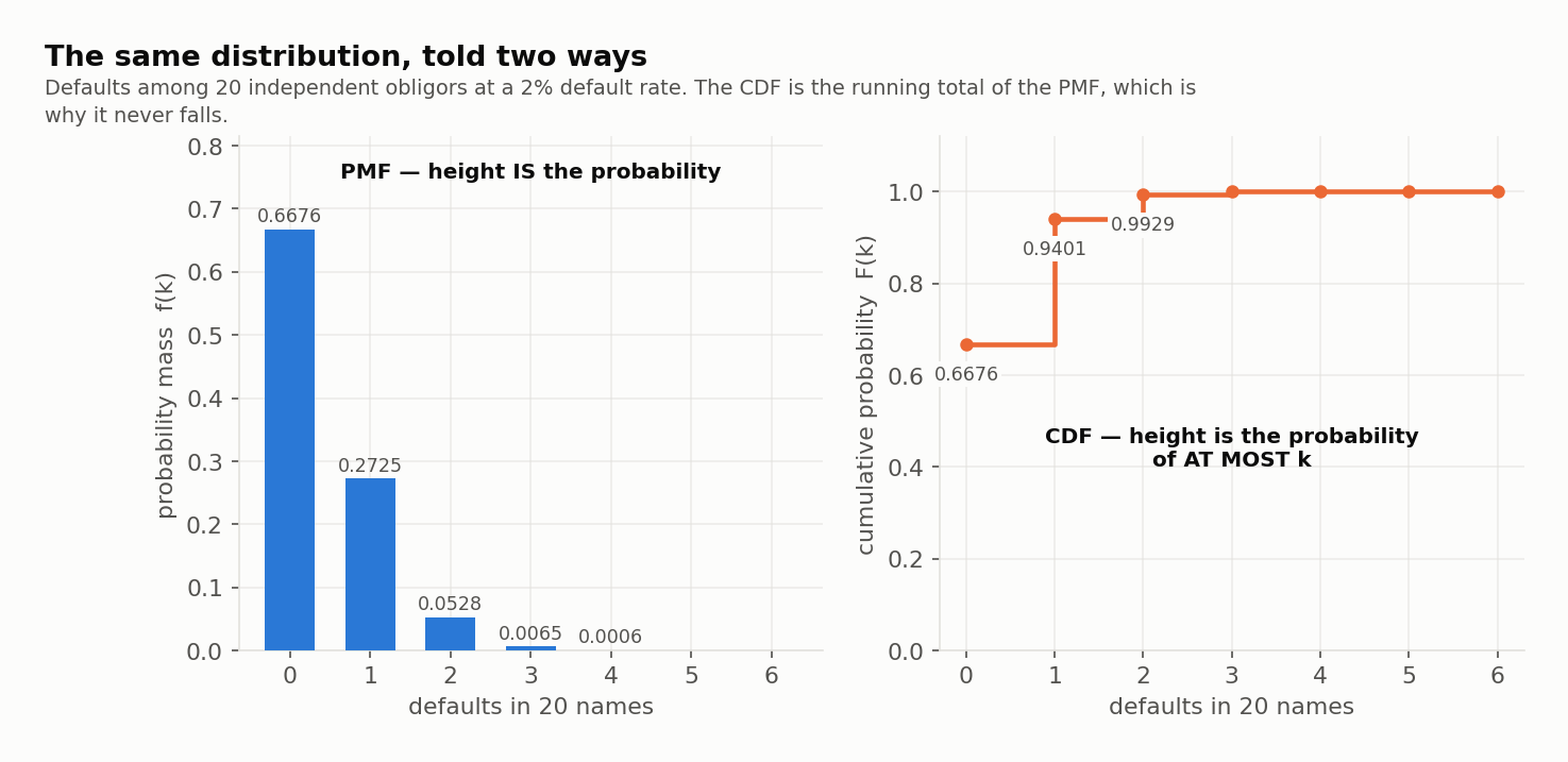
Two readings of the same object. The PMF says a single default is the most likely non-zero outcome at 27.25%. The CDF says two or fewer defaults covers 99.29% of the distribution — so three or more has probability 0.71%, which is the kind of number a concentration limit is set against.
Worked Problem — From a Mass Function to an Event and a CDF
Problem. For the 20-name portfolio, the PMF gives , , and . Compute the CDF at 0, 1, 2 and 3, the probability of one or two defaults, and the probability of three or more.
Solution.
- CDF. Running sums: , , , .
- One or two defaults. Add the masses of the outcomes in the event: — or, from the CDF, .
- Three or more. The complement of "two or fewer": .
Answer: CDF 0.6676, 0.9401, 0.9929, 0.9994; P(1 or 2) = 0.3253; P(3 or more) = 0.0071.
1.4 Bayes' Rule, and Why the Screen Is Right 15.52% of the Time
Bayes' rule inverts a conditional probability. It is the formal version of the mistake §1.2 warned about, and the reason that mistake is so expensive.
The denominator is the law of total probability: the event can arrive by two routes, and you must count both. Almost every Bayes error in practice is a forgotten second route.
Ravensmoor's model flags obligors it expects to default. The model is good: it catches 90% of the names that do default (its sensitivity), and it clears 90% of the names that do not (its specificity). The book's underlying default rate is the 2.00% from §1.2. The credit committee wants to know what a flag means.
Worked Problem — What a Flag Is Worth
Problem. The screen has 90% sensitivity and 90% specificity, applied to a book with a 2.00% default rate. An obligor is flagged. What is the probability that it actually defaults?
Solution — step by step. Work in frequencies over 10,000 obligors; it is faster than the formula and much harder to get wrong.
- Split the population. At a 2.00% rate, 200 will default and 9,800 will not.
- True positives. The screen catches 90% of the 200: .
- False positives. It wrongly flags 10% of the 9,800: .
- Total flagged. names get flagged.
- The answer. Of those, 180 genuinely default: .
Answer: 15.52%. A flag from a 90%-accurate model is wrong 84.48% of the time — more than five times out of six.
Nothing is broken. The model does exactly what it advertises. The 980 false positives simply come from a much larger pool than the 180 true positives — there are 49 healthy obligors for every defaulter, so even a 10% error rate on the healthy names swamps a 90% hit rate on the defaulters.
BA II Plus keystrokes: The Positive Predictive Value — base rate 2%, sensitivity 90%, specificity 90%, per 10,000 obligors
| Keys | Display | Note |
|---|---|---|
| 10000 × 0.02 = | → 200 | obligors that will default |
| × 0.9 = STO 1 | → 180 | true positives — park it |
| 10000 - 200 = | → 9800 | obligors that will not |
| × 0.1 = | → 980 | false positives |
| + RCL 1 = | → 1160 | everything the screen flags |
| STO 2 | park the denominator | |
| RCL 1 ÷ RCL 2 = | → 0.155172 | PPV: 15.52% |
Validation: the screen as a frequency table
# Ravensmoor's obligor default screen, as a frequency table over 10,000 names.
base, sens, spec, pop = 0.0200, 0.90, 0.90, 10_000

defaulters = pop * base
healthy = pop - defaulters
true_pos = defaulters * sens
false_pos = healthy * (1 - spec)
flagged = true_pos + false_pos

print(f"obligors                {pop:,}")
print(f"  will default          {defaulters:,.0f}")
print(f"  will not              {healthy:,.0f}")
print(f"flagged by the screen   {flagged:,.0f}")
print(f"  correctly (true +)    {true_pos:,.0f}")
print(f"  wrongly   (false +)   {false_pos:,.0f}")
print(f"P(default | flagged)    {true_pos / flagged:.6f}   = {true_pos / flagged:.2%}")
print(f"P(flagged)              {flagged / pop:.4f}")
# Output:
# obligors                10,000
#   will default          200
#   will not              9,800
# flagged by the screen   1,160
#   correctly (true +)    180
#   wrongly   (false +)   980
# P(default | flagged)    0.155172   = 15.52%
# P(flagged)              0.1160
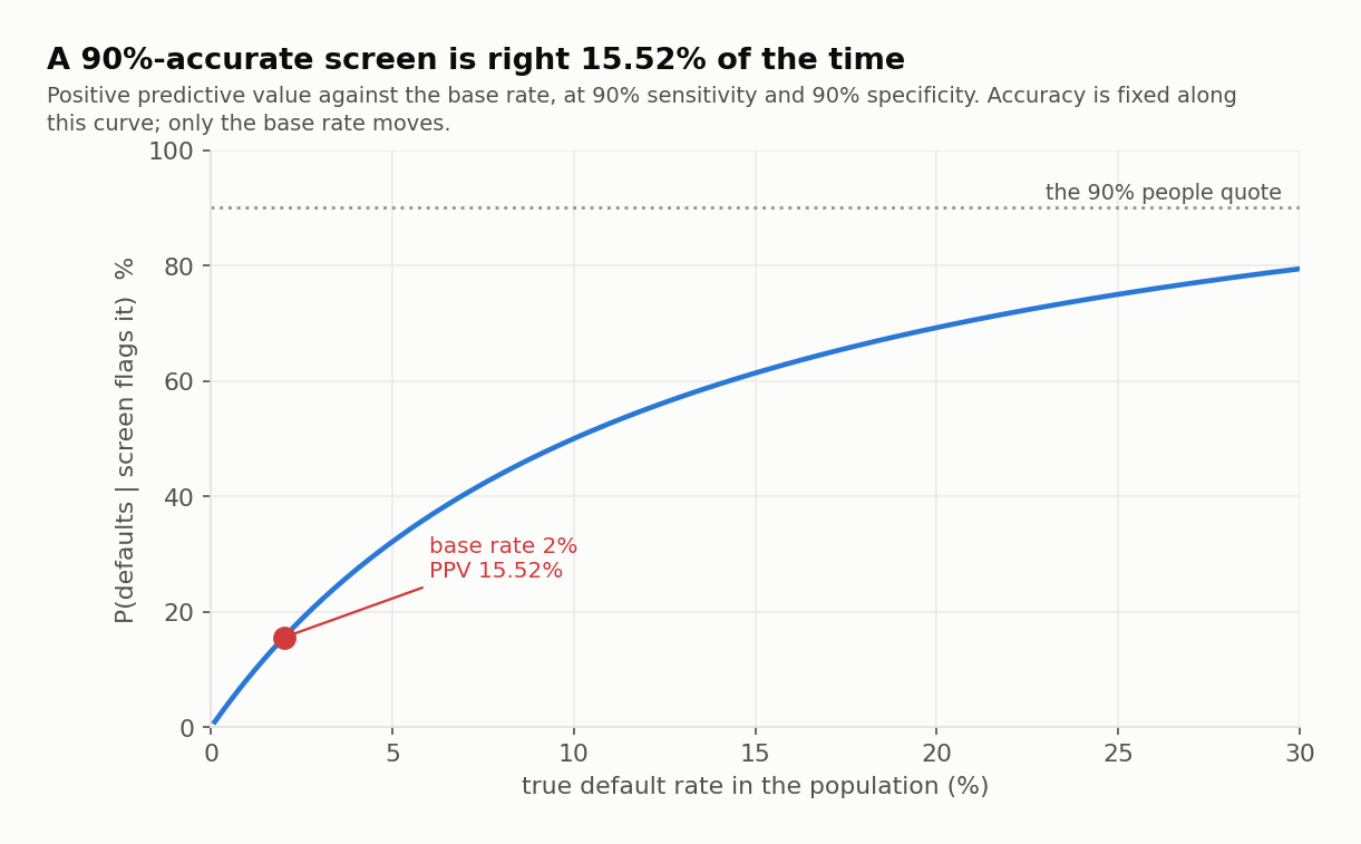
The base rate governs, and it is the number nobody quotes
Every point on that curve comes from a model with identical 90% accuracy. What changes the answer is the prevalence of the thing being detected. On a book with a 2% default rate a flag means 15.52%; on a distressed book with a 30% default rate the same model's flag means 79.41%.
This is not a statistical curiosity, it is a governance failure waiting to happen. A committee told "the model is 90% accurate" and shown a flagged name will act as though default is near-certain. The correct reading is that the name is about five and a half times likelier to survive than to fail (980 against 180), and that 980 of the 1,160 names on the report are there by mistake.
The same arithmetic returns in Chapter 8 wearing different clothes: a classifier that predicts "no default" for every obligor on this book scores 98.00% accuracy and is useless. Accuracy and base rate have to be read together or neither means anything.
1.5 Random Variables: Mass, Density and the Cumulative Function
A random variable attaches a number to each outcome, which lets the machinery of arithmetic reach the sample space.
Probability density function (PDF) For a continuous random variable, the PDF is not a probability — for every single point. It is a density: probability per unit of . Probabilities come from integrating it over an interval, so may exceed one wherever the variable is concentrated tightly enough.
That last point is the one candidates resist, and it is worth a concrete case. A uniform distribution on the interval from 0 to 0.5 has density 2 everywhere on that interval. A density of 2 is not a probability of 2; it is 2 units of probability per unit of , over an interval half a unit wide, totalling one.
Cumulative distribution function (CDF) , defined identically for discrete and continuous variables. It is non-decreasing, runs from 0 to 1, and is the object you actually use — every quantile, p-value and value-at-risk figure in this course is a statement about a CDF or its inverse.
One Object, Three Views — and Only the CDF Is Universal
- The PMF exists only for discrete variables, where its height is a probability.
- The PDF exists only for continuous variables, where its height is a density and probability is the area beneath it.
- The CDF exists for both, always means the same thing, and is what connects them: the CDF is the running sum of a PMF and the running integral of a PDF.
When a question mixes the language — "the probability that the return equals exactly 4.00%" for a continuous variable — the answer is zero, and the question is testing this distinction rather than the arithmetic.
Worked Problem — Probability From a Density
Problem. (a) is uniform on , with density 2. What is ? (b) An obligor's time to default , in years, is exponential with density and . What is the probability it defaults within five years?
Solution.
- Uniform. Probability is area under the density: .
- Exponential. .
Answer: 0.40, and 9.52%. Both are CDF values: the uniform's CDF is on the interval and the exponential's is , which is how the exam usually presents them — the integration has been done once and for all.
1.6 Expectation and the Four Population Moments
Expectation is a probability-weighted average, and it is the operator the rest of the course runs on.
The curriculum names four population moments, and the exam expects all four by name and by formula.
The mean is the centre. The variance is dispersion, in squared units — which is why the standard deviation is what gets reported. Skewness is standardised third moment: positive means a long right tail, negative a long left tail, zero a symmetric distribution. Kurtosis is standardised fourth moment and is about the tails, not the peak: the normal has exactly, and anything above that is called excess kurtosis or fat tails.
Both and are dimensionless by construction, because dividing by and cancels the units. That is what makes them comparable across a loss distribution measured in dollars and a return distribution measured in percent.
Worked Problem — Four Moments of a Quarterly Loss
Problem. Ravensmoor's operational-risk team models the quarterly loss from one process as a discrete variable: $0M with probability 0.8200, $6M with 0.1300, $12M with 0.0400 and $18M with 0.0100. Compute the mean, variance, standard deviation, skewness and kurtosis.
Solution — step by step.
- Check it is a PMF. . Good.
- Mean. , so $1.44M.
- Variance. Weight each squared deviation from 1.44: .
- Standard deviation. , so $3.41M — more than twice the mean.
- Skewness. The cubed deviations are , , and ; weighted by the probabilities they sum to . Dividing by gives 2.589583.
- Kurtosis. The fourth powers weighted by probability sum to . Dividing by gives 9.718661, an excess of 6.718661.
Answer: mean $1.44M, standard deviation $3.41M, skewness 2.5896, kurtosis 9.7187.
Read the shape rather than the numbers. The distribution is strongly right-skewed and extremely fat-tailed, which is the signature of every operational-loss series: almost all quarters cost nothing, and the average is driven by rare large events. A mean of $1.44M describes no quarter that actually occurs — the process either loses nothing, which happens 82% of the time, or loses several multiples of the mean.
BA II Plus keystrokes: Mean and Variance of a Discrete Variable — outcomes 0 / 6 / 12 / 18 with probabilities 0.82 / 0.13 / 0.04 / 0.01
| Keys | Display | Note |
|---|---|---|
| 6 × 0.13 = | → 0.78 | second outcome's contribution |
| + ( 12 × 0.04 ) = | → 1.26 | |
| + ( 18 × 0.01 ) = | → 1.44 | the mean — park it |
| STO 1 | ||
| ( 0 - RCL 1 ) x² × 0.82 = | → 1.700352 | |
| + ( ( 6 - RCL 1 ) x² × 0.13 ) = | → 4.40352 | |
| + ( ( 12 - RCL 1 ) x² × 0.04 ) = | → 8.864064 | |
| + ( ( 18 - RCL 1 ) x² × 0.01 ) = | → 11.6064 | the variance |
| √x | → 3.406817 | standard deviation |
Validation: the four moments from first principles
# The four population moments of a discrete loss variable, from first principles.
outcomes = [0.0, 6.0, 12.0, 18.0]          # $M lost in a quarter
probs    = [0.8200, 0.1300, 0.0400, 0.0100]

assert abs(sum(probs) - 1) < 1e-12, "a PMF must sum to one"

mean = sum(x * p for x, p in zip(outcomes, probs))
var  = sum((x - mean) ** 2 * p for x, p in zip(outcomes, probs))
sd   = var ** 0.5
skew = sum((x - mean) ** 3 * p for x, p in zip(outcomes, probs)) / sd ** 3
kurt = sum((x - mean) ** 4 * p for x, p in zip(outcomes, probs)) / sd ** 4

print(f"mean      {mean:.4f}")
print(f"variance  {var:.4f}")
print(f"std dev   {sd:.6f}")
print(f"skewness  {skew:.6f}")
print(f"kurtosis  {kurt:.6f}   (excess {kurt - 3:.6f})")
# Output:
# mean      1.4400
# variance  11.6064
# std dev   3.406817
# skewness  2.589583
# kurtosis  9.718661   (excess 6.718661)
1.7 Quantiles and Quantile-Based Estimators
A quantile inverts the CDF: instead of asking what probability sits below a value, it asks what value has a given probability below it.
The infimum in that definition handles the discrete case, where the CDF jumps and no value has a CDF of exactly ; for a continuous variable it is simply the inverse function. The median is , the quartiles are and , and the interquartile range is their difference.
Quantile-based estimators matter in risk work because they are robust: the median and the IQR are barely moved by an extreme observation, while the mean and standard deviation are dragged by it. That robustness is a virtue when cleaning data and a vice when measuring tail risk, because the tail is precisely what you are trying to see.
Value-at-risk is a quantile, which is the reason this section exists. The Core Equity Fund reports an 11.00% annual return and 18.00% annual volatility; to get to a monthly loss quantile, both have to be rescaled first.
Worked Problem — The Fund's Monthly Loss Quantiles
Problem. The Core Equity Fund returns 11.00% a year with a volatility of 18.00%. Assuming returns are normal and independent across months, find the monthly mean and volatility, then the 5% and 1% monthly return quantiles.
Solution — step by step.
- Monthly mean. Means scale linearly with time: .
- Monthly volatility. Variances scale linearly, so volatilities scale with the square root of time: .
- The 5% quantile. The standard normal's 5% point is : .
- The 1% quantile. The standard normal's 1% point is : .
Answer: a monthly mean of 0.9167% and volatility of 5.1962%; the 5% quantile is −7.6302% and the 1% quantile is −11.1714%.
Step 2 is where marks are lost. Dividing the volatility by 12 rather than by gives 1.50%, understating monthly risk by a factor of 3.46, and the resulting loss quantiles would be wrong by the same factor. Means scale with ; volatilities scale with .
Worked Problem — One Bad Month Against the Median
Problem. Ten monthly returns of a credit sleeve are , , , , , , , , and percent, the last from a single default. Compare the mean and median, and the standard deviation and interquartile range, with and without that month. Use positions for the quartiles.
Solution.
- Mean. The ten returns sum to , so the mean is . Without the default month: .
- Median. Sorted, the ten are ; the median averages the fifth and sixth, . Without the default month it is the fifth of nine, .
- Quartiles. The 25th percentile sits at position : . The 75th at : . The IQR is points.
- Standard deviation. With the default month, ; without it, .
Answer: one month moves the mean by 1.87 points and the standard deviation ninefold, while the median moves by 0.05. That is robustness. Whether it is a virtue depends on the question: the median describes a typical month well and says nothing about the default — which, for a credit sleeve, is the thing being measured.
The same inversion works on a discrete distribution. For the operational loss of §1.6 the CDF is at $0M, at $6M, at $12M and at $18M. The median is $0M — the CDF first reaches 0.5 there — the 95th percentile is $6M and the 99th is $12M. A quarter's typical loss is nothing; the mean of $1.44M is pulled up entirely by the tail.
1.8 Linear Transformations, and What They Leave Alone
Risk work is full of linear transformations: converting a currency, deducting a fee, levering a position, standardising a variable. For the effects are completely determined.
Three patterns carry the whole table. The shift moves location and nothing else — mean, median and quantiles all move by , while every measure of spread and shape is untouched. The scale multiplies spread but enters the variance squared, and the absolute value matters because a standard deviation cannot be negative. Shape is scale-free: skewness and kurtosis are unchanged, except that a negative flips the sign of skewness by reflecting the distribution.
Worked Problem — A Management Fee Is a Shift, Not a Scaling
Problem. The Core Equity Fund charges a flat management fee of 1.20% a year, accrued monthly, deducted from the gross return. Using the monthly figures from §1.7, state the net monthly mean, volatility and 5% quantile.
Solution — step by step.
- Identify the transformation. Net gross fee, so with and .
- Mean. .
- Volatility. Since , volatility is unchanged at .
- 5% quantile. The quantile shifts by along with everything else: .
Answer: mean 0.8167%, volatility 5.1962% unchanged, 5% quantile −7.7302%.
A flat fee makes the fund worse without making it any less volatile, so every risk-adjusted ratio falls — the numerator drops and the denominator does not. A performance fee behaves entirely differently, because it is a function of the return rather than a constant, and therefore is not a linear transformation at all.
Worked Problem — Rescaling a Skewed Loss, and Turning It Upside Down
Problem. The quarterly operational loss of §1.6 has mean $1.44M, standard deviation $3.4068M, skewness 2.5896, kurtosis 9.7187, median $0M and 95th percentile $6M. (a) A subsidiary's loss is modelled as : a quarter more exposure plus a fixed $0.40M of handling cost. Give the same six figures for . (b) A reinsurer that pays the whole loss sees its own result as . What happens to the skewness and kurtosis?
Solution.
- Mean and median shift and scale. Mean , so $2.20M; median , so $0.40M.
- Spread scales by only. Standard deviation , so $4.2585M; the 95th percentile, a quantile, moves with the line: , so $7.90M.
- Shape is untouched. Skewness and kurtosis are dimensionless and , so they stay at 2.5896 and 9.7187.
- Reversing the sign. For , : the standard deviation is still $3.4068M, the kurtosis still 9.7187, but the skewness becomes −2.5896, because the long tail now points the other way.
Answer: mean $2.20M, sd $4.2585M, median $0.40M, 95th percentile $7.90M, skewness and kurtosis unchanged; for the reinsurer, skewness flips to −2.5896 and nothing else about the shape changes. The fixed handling cost is the part candidates mis-handle: it shifts every location measure and touches no measure of spread or shape.
BA II Plus keystrokes: Monthly Scaling and a Fee — annual return 11.00%, annual volatility 18.00%, fee 1.20% a year
| Keys | Display | Note |
|---|---|---|
| 11 ÷ 12 = | → 0.916667 | monthly mean — means scale with t |
| STO 1 | ||
| 18 ÷ 12 √x = | → 5.196152 | monthly vol — scales with root t |
| STO 2 | ||
| 1.644854 +/- × RCL 2 = | → -8.546912 | |
| + RCL 1 = | → -7.630245 | the 5% quantile (−7.630243 with z to more places) |
| - ( 1.2 ÷ 12 ) = | → -7.730245 | after the fee, a pure shift (−7.730243 with z to more places) |
Validation: scaling, quantiles and the fee
# The fund's monthly moments, a normal quantile, and what a fee does to them.
from scipy.stats import norm

r_ann, vol_ann = 11.00, 18.00
r_m = r_ann / 12
vol_m = vol_ann / 12 ** 0.5

print(f"monthly mean        {r_m:.6f}%")
print(f"monthly volatility  {vol_m:.6f}%")
for p in (0.05, 0.01):
    print(f"{p:.0%} quantile        {r_m + norm.ppf(p) * vol_m:.6f}%")

# a flat fee of 1.20% a year, charged monthly: Y = a + bX with a = -0.10, b = 1
fee_m = 1.20 / 12
print()
print(f"after a {fee_m:.2f}% monthly fee:")
print(f"  mean              {r_m - fee_m:.6f}%   (shifts by the fee)")
print(f"  volatility        {vol_m:.6f}%   (UNCHANGED - a shift is not a scaling)")
print(f"  5% quantile       {r_m - fee_m + norm.ppf(0.05) * vol_m:.6f}%")
# Output:
# monthly mean        0.916667%
# monthly volatility  5.196152%
# 5% quantile        -7.630243%
# 1% quantile        -11.171391%
#
# after a 0.10% monthly fee:
#   mean              0.816667%   (shifts by the fee)
#   volatility        5.196152%   (UNCHANGED - a shift is not a scaling)
#   5% quantile       -7.730243%
1.9 The Distributions the Curriculum Names
The syllabus lists eleven distributions by name and expects their properties and applications. Rather than eleven definitions to memorise, carry three questions: what is the support, what does it count or measure, and where does it show up in risk work.
| Distribution | Support | What it models | Where it appears |
|---|---|---|---|
| Bernoulli | one trial with two outcomes | a single obligor defaulting | |
| Binomial | 0, 1, …, n | successes in independent trials | defaults in a homogeneous pool |
| Poisson | 0, 1, 2, … | events in a fixed interval at a constant rate | operational-loss event counts |
| Uniform | every value equally likely | pseudo-random number generation | |
| Normal | sums of many small independent shocks | the CLT's limit; return modelling | |
| Lognormal | a variable whose log is normal | asset prices, which cannot go negative | |
| Chi-squared | sum of squared standard normals | variance tests; the Jarque-Bera statistic | |
| Student's t | a normal mean with an estimated variance | small-sample tests; fat-tailed returns | |
| F | ratio of two scaled chi-squared variables | joint restrictions in regression | |
| Exponential | waiting time between Poisson events | time to default | |
| Beta | a proportion or probability | recovery rates and loss given default |
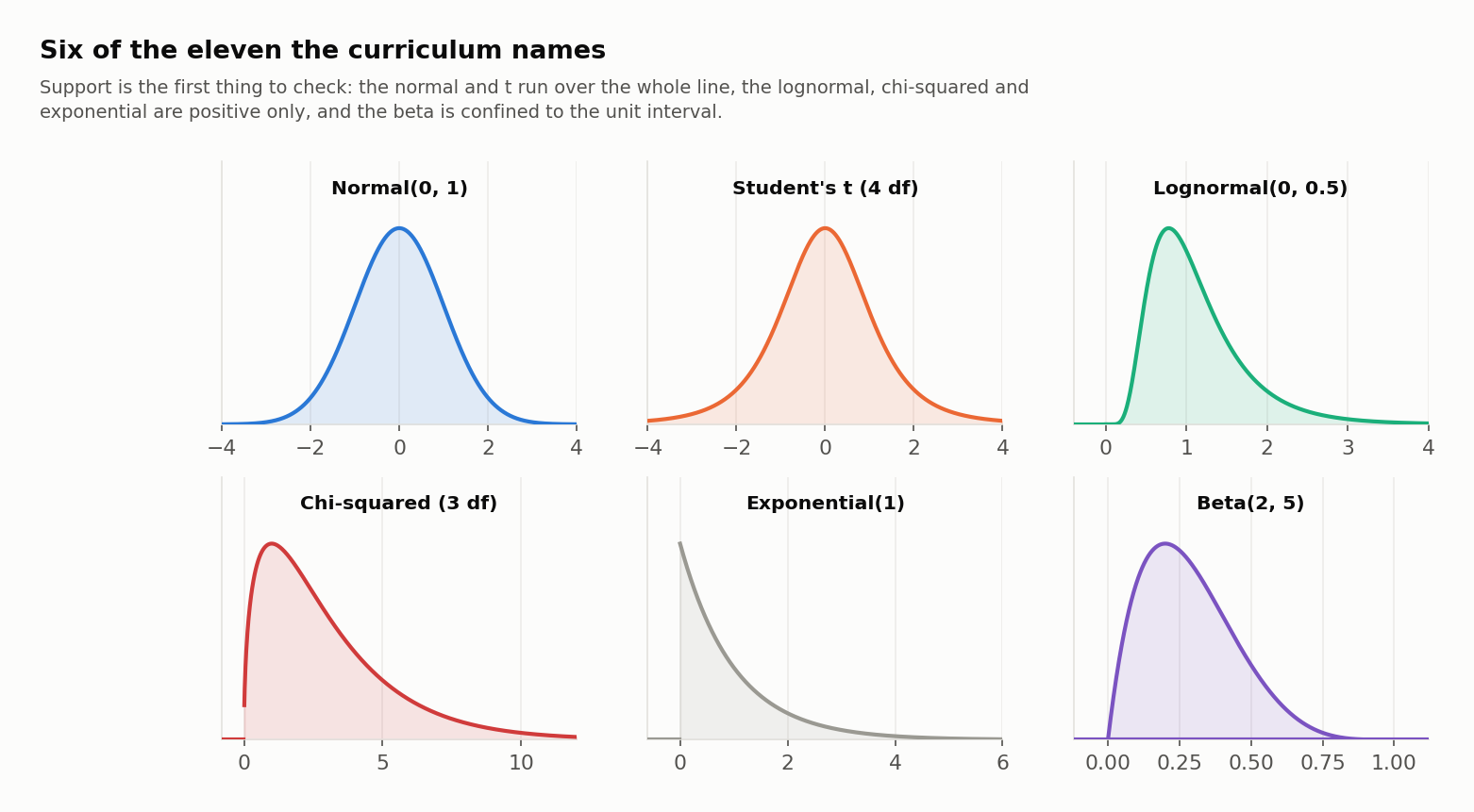
Four relationships the exam tests more often than the definitions
- Bernoulli sums to binomial. independent Bernoulli trials with the same give a binomial. Independence is the assumption that fails on a real loan book.
- Binomial tends to Poisson. For large and small with fixed, the binomial converges to a Poisson with . The 20-name portfolio of §1.3 at is already close.
- Exponential is the Poisson waiting time. If events arrive Poisson at rate , the gap between them is exponential with mean . The exponential is memoryless, which is both its convenience and its least realistic feature.
- Student's t tends to normal. As degrees of freedom rise the t converges to the normal; below about 30 its fatter tails matter, which is exactly the small-sample case Chapter 3 tests in.
Parameters and moments
The exam asks for the mean and variance of each named distribution far more often than for its density.
| Distribution | Parameters | Mean | Variance |
|---|---|---|---|
| Bernoulli | |||
| Binomial | |||
| Poisson | |||
| Uniform | |||
| Normal | |||
| Lognormal | of | ||
| Chi-squared | degrees of freedom | ||
| Student's t | degrees of freedom | (for ) | (for ) |
| F | (for ) | depends on both; finite for | |
| Exponential | rate | ||
| Beta |
Three of these carry the calculations the exam sets most often. The Poisson probability of events is . A normal probability is found by standardising, , and reading . An exponential time has and a median of .
Worked Problem — A Poisson Count, a Normal Tail and an Exponential Median
Problem. (a) Operational-loss events arrive at an average of 3 a quarter, Poisson. What is the probability of no events, and of five or more? (b) The fund's monthly return is normal with mean and volatility . Given , what is the probability of losing more than 5% in a month? (c) A time to default is exponential with a year. What are its mean and median?
Solution.
- Poisson, zero. .
- Poisson, five or more. The complement of four or fewer. The masses for 0 to 4 are , , , and — each the previous one times — summing to . So .
- Normal. , and : a 12.74% chance in any month.
- Exponential. Mean years; median years. The median is well below the mean, because the exponential is right-skewed.
Answer: 4.98% and 18.47%; 12.74%; mean 50 years, median 34.66 years.
BA II Plus keystrokes: Poisson Probabilities by Recursion — lambda = 3; P(k) = P(k - 1) x 3 / k
| Keys | Display | Note |
|---|---|---|
| 3 +/- 2nd eˣ | → 0.049787 | P(0) |
| STO 1 × 3 = | → 0.149361 | P(1) |
| STO + 1 × 3 ÷ 2 = | → 0.224042 | P(2), and add P(1) to memory |
| STO + 1 × 3 ÷ 3 = | → 0.224042 | P(3) |
| STO + 1 × 3 ÷ 4 = | → 0.168031 | P(4) |
| STO + 1 RCL 1 | → 0.815263 | P(4 or fewer) |
| +/- + 1 = | → 0.184737 | P(5 or more) |
Worked Problem — A Price, a Recovery Rate and a Default Count
Problem. (a) A price relative (one year's price divided by today's) is lognormal, with normal with mean 0.05 and standard deviation 0.20. Find the mean and median of , and the probability the price falls, given . (b) A recovery rate is beta with and . Find its mean and standard deviation. (c) Fifteen independent obligors each default with probability 3.00%. Find the expected number of defaults, its variance, and the probability of two or more.
Solution.
- Lognormal mean. — a 7.25% expected gain.
- Lognormal median. , below the mean: the lognormal is right-skewed, so its mean is pulled above its median by the long upper tail.
- Price falls. exactly when , so .
- Beta. Mean ; variance , so the standard deviation is . A beta is bounded by 0 and 1, which is why it suits a recovery rate.
- Binomial moments. Mean ; variance .
- Two or more. and , so .
Answer: lognormal mean 1.0725, median 1.0513, P(fall) 40.13%; beta mean 0.40, sd 0.20; binomial mean 0.45, variance 0.4365, P(2 or more) 7.30%. The lognormal result is the one candidates miss: an asset with an expected gain of 7.25% finishes below where it started 40% of the time, and half the time it gains less than 5.13% — the mean is not the typical outcome.
BA II Plus keystrokes: Lognormal and Binomial — ln X ~ N(0.05, 0.20); binomial n = 15, p = 0.03
| Keys | Display | Note |
|---|---|---|
| 0.2 x² ÷ 2 + 0.05 = 2nd eˣ | → 1.072508 | lognormal mean |
| 0.05 2nd eˣ | → 1.051271 | lognormal median |
| 0.97 y^x 15 = | → 0.633251 | P(0 defaults) |
| STO 1 | ||
| 0.97 y^x 14 × 0.45 = | → 0.293776 | P(1 default) |
| + RCL 1 = +/- + 1 = | → 0.072972 | P(2 or more) |
Validation: the probability rules and the named distributions
import numpy as np
from math import exp, log
from scipy import stats

print(f"P(SG or D)          {0.30 + 0.02 - 0.016:.4f}")
print(f"P(at least 1 of 2)  {1 - 0.98 ** 2:.4f}")
print(f"P(D), total prob.   {0.004 / 0.70 * 0.70 + 0.016 / 0.30 * 0.30:.4f}")
b = stats.binom(20, 0.02)
print(f"binomial CDF        {b.cdf(0):.4f} {b.cdf(1):.4f} {b.cdf(2):.4f} {b.cdf(3):.4f}")
print(f"P(1 or 2 defaults)  {b.pmf(1) + b.pmf(2):.4f}   P(3+) {b.sf(2):.4f}")
print(f"exponential P(T<=5) {1 - exp(-0.02 * 5):.6f}   median {log(2) / 0.02:.2f}")
po = stats.poisson(3)
print(f"Poisson P(0) {po.pmf(0):.6f}   P(<=4) {po.cdf(4):.6f}   P(>=5) {po.sf(4):.6f}")
z = (-5 - 11.00 / 12) / (18.00 ** 2 / 12) ** 0.5
print(f"normal z {z:.4f}   P(R < -5%) {stats.norm.cdf(z):.4f}")
r = np.array([1.2, 0.8, -0.5, 1.5, 0.9, 1.1, -0.3, 0.6, 1.0, -18.0])
print(f"ten months: mean {r.mean():.2f}  median {np.median(r):.2f}  sd {r.std(ddof=1):.2f}")
print(f"nine months: mean {r[:-1].mean():.2f}  median {np.median(r[:-1]):.2f}  sd {r[:-1].std(ddof=1):.2f}")
print(f"lognormal mean {exp(0.07):.4f}  median {exp(0.05):.4f}  P(X<1) {stats.norm.cdf(-0.25):.4f}")
print(f"beta(2,3) mean {2 / 5:.2f}  sd {(6 / 150) ** 0.5:.2f}")
bi = stats.binom(15, 0.03)
print(f"binomial(15, 3%) P(0) {bi.pmf(0):.4f}  P(1) {bi.pmf(1):.4f}  P(2+) {bi.sf(1):.4f}")
# Output:
# P(SG or D)          0.3040
# P(at least 1 of 2)  0.0396
# P(D), total prob.   0.0200
# binomial CDF        0.6676 0.9401 0.9929 0.9994
# P(1 or 2 defaults)  0.3253   P(3+) 0.0071
# exponential P(T<=5) 0.095163   median 34.66
# Poisson P(0) 0.049787   P(<=4) 0.815263   P(>=5) 0.184737
# normal z -1.1387   P(R < -5%) 0.1274
# ten months: mean -1.17  median 0.85  sd 5.95
# nine months: mean 0.70  median 0.90  sd 0.67
# lognormal mean 1.0725  median 1.0513  P(X<1) 0.4013
# beta(2,3) mean 0.40  sd 0.20
# binomial(15, 3%) P(0) 0.6333  P(1) 0.2938  P(2+) 0.0730
1.10 Mixture Distributions: Two Normal Regimes, No Normality
The last outcome in this chapter is the one that does the most work later. A mixture draws from one of several component distributions, with fixed probabilities deciding which.
Mixture distribution A distribution whose density is a probability-weighted sum of component densities, with weights summing to one. The mixture is a single, valid distribution — not a portfolio of them — and its shape need not resemble any component.
Markets are the obvious application: a calm regime most of the time, a stressed regime occasionally. Suppose Ravensmoor models the fund as calm 90% of months and stressed 10%, both regimes centred on zero. For a zero-mean mixture the variance is the weighted average of component variances, and the fourth moment is the weighted average of component fourth moments.
The factor of 3 in the numerator is each normal component's own kurtosis. Notice what that means: if every component has the same variance the expression collapses to exactly 3, and the mixture is no fatter-tailed than a normal. All of the excess kurtosis comes from the components differing.
Worked Problem — Calibrating a Regime Mixture to the Fund
Problem. Model the fund's monthly return as a mixture: a calm regime with 4.00% volatility 90% of the time, and a stressed regime the other 10%. Choose the stressed volatility so that the mixture reproduces the fund's own monthly volatility of 5.196152%. Then find the mixture's kurtosis.
Solution — step by step.
- Set up the variance condition. .
- Solve for the stressed variance. , so and .
- Stressed volatility. — a little over 2.8 times the calm regime.
- Kurtosis. The numerator is ; the denominator is . So .
Answer: a stressed volatility of 11.2250% gives a mixture with kurtosis 7.4815 against the normal's 3.
Validation: the mixture's volatility, kurtosis and tail
# Two normal regimes whose mixture reproduces the fund's monthly volatility.
from scipy.stats import norm

vol_m = 18.00 / 12 ** 0.5
w, s_calm = 0.10, 4.00
s_stress = ((vol_m ** 2 - (1 - w) * s_calm ** 2) / w) ** 0.5

var = (1 - w) * s_calm ** 2 + w * s_stress ** 2
kurt = 3 * ((1 - w) * s_calm ** 4 + w * s_stress ** 4) / var ** 2

print(f"stressed-regime vol  {s_stress:.6f}%")
print(f"mixture volatility   {var ** 0.5:.6f}%   (the fund's {vol_m:.6f}%)")
print(f"mixture kurtosis     {kurt:.6f}   (each component is 3)")

def mix_cdf(x):
    return (1 - w) * norm.cdf(x, 0, s_calm) + w * norm.cdf(x, 0, s_stress)

lo, hi = -60.0, 60.0
for _ in range(200):
    mid = (lo + hi) / 2
    lo, hi = (mid, hi) if mix_cdf(mid) < 0.01 else (lo, mid)
q_mix = (lo + hi) / 2
q_norm = norm.ppf(0.01, 0, var ** 0.5)

print(f"1% mixture quantile  {q_mix:.6f}%")
print(f"1% normal quantile   {q_norm:.6f}%")
print(f"the normal is short by {abs(q_mix) - abs(q_norm):.6f} pp")
# Output:
# stressed-regime vol  11.224972%
# mixture volatility   5.196152%   (the fund's 5.196152%)
# mixture kurtosis     7.481481   (each component is 3)
# 1% mixture quantile  -14.471310%
# 1% normal quantile   -12.088058%
# the normal is short by 2.383252 pp
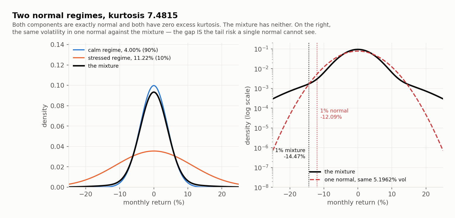
A mixture of normals is not normal, and the error is one-directional
Both regimes here are perfectly normal. Neither has a single unit of excess kurtosis. Mix them and kurtosis is 7.4815 — and the mixture has exactly the same 5.196152% volatility as the single normal it is being compared against.
So volatility cannot distinguish them. The 1% quantile can: −14.4713% for the mixture against −12.0881% for the normal, a shortfall of 2.3833 percentage points. A risk system that fits one normal to this fund gets the volatility exactly right and understates the 1-in-100 month by nearly a quarter of it.
The direction of the error depends on how far into the tail you look. Holding the variance fixed, regime-switching moves probability into the far tails and takes it from the shoulders, so the mixture is less extreme than the normal at a 5% quantile and much more extreme at 1% (Chapter 7, §7.3, shows both). For the extreme quantiles that set capital and limits, a normal assumption on a market with regimes is not merely imprecise — it is systematically optimistic about the far tail. Chapter 7 tests the fund's actual returns for exactly this with the Jarque-Bera statistic, and Chapter 3's confidence intervals are built on the normal assumption this section has just undermined.
1.11 Putting It All Together
Ravensmoor's credit committee and its risk function both meet this week, and each has a question this chapter answers.
The problem. The committee has a report listing 1,160 flagged obligors and wants to know how seriously to take it. The risk function has a fund reporting 18.00% volatility and wants a 1-in-100 month.
Why this step: establish what a flag means. From §1.4, the screen's 90% accuracy applied to a 2.00% base rate gives a positive predictive value of 15.52%. Of the 1,160 names, about 180 will default and 980 will not. The report is not a list of failures; it is a shortlist that is wrong six times out of seven, and it should drive a review rather than a provision.
Why this step: convert the fund's annual numbers to a monthly distribution. From §1.7, means scale with time and volatilities with its square root: 0.916667% and 5.196152% a month. Under a normal assumption the 1% quantile is −11.171391%.
Why this step: ask whether the normal assumption survives. From §1.10, a calm/stressed mixture with the same 5.196152% volatility puts the zero-mean 1% quantile at −14.471310% against the normal's −12.088058%. The volatility is identical and the tail is not.
The answer. The flag list means far less than it appears to, and the fund's tail means considerably more. Both conclusions come from the same move: asking what the conditional distribution is, rather than reading an unconditional headline. A 90% accuracy is unconditional on the base rate; an 18.00% volatility is unconditional on the regime. Conditioning changes both answers, and in opposite directions.
- 180 of 1,160 Flagged names that will actually default (the other 980 are the screen's false positives)
- -11.17% 1% monthly quantile under one normal (from 0.9167% mean, 5.1962% volatility)
- -14.47% 1% quantile once regimes are allowed (zero mean) (against -12.09% for a zero-mean normal of the same volatility: 2.38pp deeper)
Chapter Summary
What You Learned in Chapter 1
- Mutually exclusive and independent are nearly opposites. Mutually exclusive events cannot co-occur and are therefore maximally dependent; independent events satisfy . Two events with non-zero probability cannot be both.
- A conditional probability renormalises onto what is known, and is not . On Ravensmoor's book, while — the same cell, different denominators.
- Conditional independence is the assumption behind every factor model. Obligors are dependent unconditionally and usually modelled as independent given the economy; the conditioning variable carries the correlation.
- Bayes' rule inverts a conditional, and the base rate governs the answer. A screen with 90% sensitivity and 90% specificity on a 2.00% book yields a positive predictive value of 15.52% — 180 true positives against 980 false ones. Nothing is wrong with the model.
- PMF, PDF and CDF are three views of one object. A PMF's height is a probability; a PDF's height is a density and may exceed one; the CDF exists for both and is what quantiles, p-values and VaR are actually built on.
- Four population moments: mean, variance, skewness and kurtosis, the last two dimensionless by construction. The normal has kurtosis exactly 3. Ravensmoor's operational loss has skewness 2.5896 and kurtosis 9.7187 on a mean of $1.44M, which is the signature of a loss series where the average describes no quarter that occurs.
- A quantile inverts the CDF, and value-at-risk is a quantile. Means scale with and volatilities with : the fund's 18.00% annual volatility is 5.196152% monthly, not 1.50%.
- Under the shift moves location only; the scale multiplies spread and enters variance squared; skewness and kurtosis are scale-free, with flipping skewness. A flat fee is a shift, so it lowers every risk-adjusted ratio without changing volatility at all.
- Eleven distributions, three questions each — support, what it models, where it appears. Bernoulli sums to binomial, binomial tends to Poisson, exponential is the Poisson waiting time, and Student's t tends to normal.
- A mixture of normals is not normal. Two perfectly normal regimes, calibrated to the fund's own 5.196152% volatility, produce kurtosis 7.4815 and push the 1% quantile from −12.0881% to −14.4713%. Volatility cannot tell the two apart; the tail can.
What's Next
Chapter 1 worked with one random variable at a time. Chapter 2 introduces the second one, and with it covariance, correlation, and the variance of a weighted sum — the identity that decides whether a portfolio diversifies. It is the same identity Foundations used to put the loan book's unexpected loss twenty-fold apart depending on a single correlation assumption, and here it is derived rather than asserted.
Continue to Chapter 2: Multivariate Random Variables and Portfolio Moments
Concept Checks
Fast recall before the exam-format questions — no calculator needed.
-
Two events each have a probability strictly between zero and one. A risk analyst states that they are both mutually exclusive and independent. This claim is:
- Consistent, because mutual exclusivity is a restriction on which outcomes may co-occur while independence is a restriction on information, and the two restrictions operate on different objects entirely
- Consistent only if the two events have exactly equal probabilities and partition the sample space between them
- Impossible, because mutual exclusivity forces the joint probability to zero while independence requires it to be positive
- Impossible, because independence requires that the two events have no outcomes in common by definition
-
A credit model reports that the probability an obligor is speculative grade given that it defaulted is 80%. A committee member concludes that speculative-grade obligors default 80% of the time. This conclusion is:
- Wrong, because it transposes the conditional — the two statements divide the same joint probability by different totals
- Wrong, because a conditional probability describes a long-run frequency across a population and therefore cannot be attached to any individual obligor, only to the portfolio as a whole
- Correct, because conditional probabilities are symmetric whenever the conditioning event is observable
- Correct, provided the proportion of speculative-grade obligors in the book equals the overall default rate
-
Two obligors are each followed for a year, and each either defaults or does not. Which statement about the sample space and the event space is correct?
- The sample space has two outcomes, default and survival, because each obligor can only do one of the two
- The event space has four members, one for each combination of the two obligors' outcomes over the year
- The sample space and the event space are the same set, since every outcome is also an event that can be assigned a probability
- The sample space has four outcomes, and the event space holds all sixteen subsets of them, empty set included
-
Two obligors' defaults are modelled as independent conditional on the state of the economy, but dependent unconditionally. This combination is:
- Contradictory, since conditional independence is a strictly stronger requirement that implies unconditional independence
- Coherent, and it is the standard structure of a factor model — the conditioning variable carries the correlation between the names
- Coherent only when the economy is modelled as a discrete variable taking finitely many states, since conditioning on a continuous factor leaves a residual dependence that cannot be removed
- Contradictory, because two variables that are dependent cannot become independent under any conditioning
-
A screening model has 90% sensitivity and 90% specificity. Moving it from a book with a 2% default rate to a book with a 30% default rate will:
- Raise the probability that a flagged obligor defaults, because the base rate rather than the accuracy drives that probability
- Leave the probability that a flagged obligor defaults unchanged, because the model's accuracy has not changed
- Lower the probability that a flagged obligor defaults, because more defaulters means proportionally more false positives
- Leave the probability that a flagged obligor defaults unchanged, because sensitivity and specificity are equal to each other
-
A portfolio's returns are transformed by Y = a + bX, where a is a non-zero constant and b equals one. Which quantity is unchanged?
- The mean, because adding a constant leaves the probability weights attached to each outcome untouched
- The median, because order statistics are determined by ranks rather than by the values themselves
- The standard deviation, because a shift relocates the distribution without altering any deviation from the mean
- The 5% quantile, because quantiles are defined by cumulative probability rather than by the values attained
-
Which pairing of a distribution with its support is correct?
- The lognormal distribution is defined over the entire real line, which is why it is used to model asset returns
- The beta distribution is confined to the interval from zero to one, which is why it is used to model recovery rates
- The chi-squared distribution is defined over the entire real line, which is why it is used to model test statistics
- The exponential distribution is confined to the interval from zero to one, which is why it is used to model probabilities
-
Operational-loss event counts are modelled as Poisson with an average of 4 events a quarter. Which statement is correct?
- The variance of the count is 16, because the variance of any count is the square of its mean
- The probability of no events is zero, because a Poisson variable with a positive mean must record at least one event
- The time between events is normally distributed, because counts and waiting times share the same distribution
- The variance of the count is also 4, because a Poisson distribution's mean and variance are equal
-
An analyst converts an annual volatility to a monthly figure by dividing it by twelve. The resulting monthly volatility is:
- Understated, because volatilities scale with the square root of time, so the divisor should have been the square root of twelve
- Overstated, because volatilities scale with the square of time rather than its root, so the correct divisor is one hundred and forty-four and the analyst has applied far too small a one
- Correct, because volatility and the mean are both expressed per unit of time and therefore scale identically
- Understated, because volatility does not scale with time at all and the annual figure should have been used unchanged
-
The cumulative distribution function of a discrete random variable is best described as:
- A continuous increasing curve, because cumulative probability accumulates smoothly regardless of the underlying variable
- A function that may decrease over some ranges whenever the probability mass function decreases over those ranges
- A step function that is non-decreasing everywhere, jumping at each attainable value by that value's probability mass
- A function defined only at the attainable values, and therefore undefined between consecutive outcomes
Exam-Style Practice
Ten questions at the live exam's pace of 2.4 minutes each. Four options, one best answer, calculator permitted.
Chapter 1 — Probability, Random Variables and Distributions
-
A bank's early-warning model flags obligors it expects to default. The model correctly flags 85% of obligors that go on to default and correctly clears 92% of those that do not. The underlying default rate in the portfolio is 4.00%. An obligor has just been flagged. The probability that it defaults within the year is closest to:
- 3.40%
- 30.69%
- 85.00%
- 11.08%
-
For two events A and B, the joint probability P(A and B) is 0.12, P(B) is 0.30 and P(A) is 0.20. The conditional probability P(B | A) is closest to:
- 0.40
- 0.12
- 0.30
- 0.60
-
A quarterly operational loss takes the value $0 million with probability 0.85, $5 million with probability 0.12 and $15 million with probability 0.03. The standard deviation of the quarterly loss is closest to:
- $2.94 million
- $8.65 million
- $1.05 million
- $6.67 million
-
An equity portfolio has an annual volatility of 24.00%. Assuming returns are independent across periods, the portfolio's quarterly volatility is closest to:
- 24.00%
- 4.90%
- 12.00%
- 6.00%
-
A fund's monthly returns are normally distributed with a mean of 0.60% and a volatility of 4.50%. The 5% monthly return quantile is closest to:
- -9.87%
- -8.22%
- -7.40%
- -6.80%
-
A random variable X has a standard deviation of 8.00, a skewness of -0.40 and a kurtosis of 5.00. A new variable is defined as Y = -2 + 1.5X. The standard deviation, skewness and kurtosis of Y are respectively closest to:
- 12.00, -0.60 and 7.50
- 12.00, -0.40 and 5.00
- 10.00, -0.40 and 5.00
- 12.00, 0.40 and 5.00
-
Monthly returns are modelled as a mixture of two zero-mean normal distributions: a calm regime with 3.00% volatility occurring 85% of the time, and a stressed regime with 9.00% volatility occurring 15% of the time. The volatility of the mixture is closest to:
- 3.90%
- 6.00%
- 4.45%
- 19.80%
-
A sub-portfolio holds 15 obligors whose defaults are independent, each with a one-year default probability of 3.00%. The probability that exactly one obligor defaults during the year is closest to:
- 29.38%
- 45.00%
- 63.33%
- 92.70%
-
An analyst states that for a continuous random variable the probability density function evaluated at a point gives the probability of observing that point. The statement is:
- Correct, provided the density has been normalised so that it integrates to one over its support
- Incorrect: the probability of any single point is zero, and the density is probability per unit of the variable
- Correct, provided the density never exceeds one anywhere on its support
- Incorrect: the density gives the probability of observing a value at or below that point, which is a cumulative probability
-
A fund reports an annual return of 8.40% and an annual volatility of 15.00%. It introduces a flat management fee of 1.80% a year, deducted from the gross return. Relative to the gross series, the net series has:
- A lower mean and a lower volatility, since the fee reduces both the level and the dispersion of the return
- The same mean and a lower volatility, since a fee removes a fixed amount of variability each period
- A lower mean and a lower Sharpe ratio, with volatility unchanged at 15.00%
- A lower mean and an unchanged Sharpe ratio, since the fee scales the numerator and denominator alike