Free sample chapter from FRM Level I: Foundations of Risk Management.
Chapter 1: The Building Blocks of Risk Management
Chapter 1: The Building Blocks of Risk Management
Risk management has a vocabulary problem. Almost every word in it — risk, exposure, loss, capital — is also an ordinary English word, and the ordinary meanings are close enough to the technical ones to feel safe and wrong enough to cost you marks. This chapter fixes the vocabulary, and it does so by making every term do work on a single set of numbers you will still be using in Chapter 7.
Our subject is Ravensmoor Financial Group, a mid-sized bank holding company. Ravensmoor's commercial lending division holds 400 loans of $6 million each — $2,400 million of exposure — and its chief risk officer, Ingrid Halvorsen, has been asked by the board a question that sounds simple: how much could this book lose?
There is no single answer. By the end of this chapter you will have produced three defensible ones that differ by a factor of twenty, and you will understand exactly which assumption separates them. That gap is not a failure of the arithmetic. It is the reason the discipline exists.
- $19.44M Expected loss on the book (400 loans of $6M at PD 1.80%, LGD 45%)
- 20x Spread in unexpected loss ($8.23M at zero correlation, $164.61M at one)
- $161.75M Economic capital at 99.9% (against $23.19M of unexpected loss)
Learning Objectives
Learning objectives
- State what risk is, and distinguish risk management from both risk avoidance and risk taking
- Classify the tools of risk management into quantitative measures, qualitative techniques, and enterprise-wide procedures
- Compute expected loss as EAD x PD x LGD and explain why it is priced into the spread rather than held against capital
- Compute the unexpected loss of a single exposure and interpret the ratio of unexpected to expected loss
- Explain why summing unexpected losses across a portfolio assumes perfect correlation, and compute the independent-default alternative
- Interpret the risk-reward relationship and identify the conflicts of interest that bend risk decisions
- Describe the eight major risk classes with a concrete example of each and assess their potential impact
- Explain how a shock in one risk class becomes a shock in another, and why aggregating risk is harder than adding it
1.1 What Risk Is, and What Managing It Means
Start with the definition, because the exam does.
Risk Exposure to uncertainty about a future outcome that matters. Two conditions must hold: the outcome must be uncertain, and the firm must be exposed to it. An uncertain event you are not exposed to is somebody else's risk; a certain loss you are exposed to is not a risk but a cost.
Notice what the definition does not say. It does not say risk is the possibility of loss. Uncertainty runs in both directions, and a great deal of confusion in practice comes from firms that measure only the downside and then act surprised when the upside fails to arrive either. It also does not say risk is bad. A bank that took no credit risk would hold no loans, earn no spread, and go out of business with an immaculate risk report.
That gives us the distinction the curriculum cares about most.
Risk Taking Is Not the Opposite of Risk Management
Risk taking is the deliberate acceptance of exposure in exchange for expected reward. It is what a financial institution is for. Ravensmoor takes credit risk because borrowers pay a spread over its funding cost.
Risk management is the set of activities that make risk taking deliberate rather than accidental: identifying exposures, measuring them, deciding which to keep, pricing the ones you keep, and building the capacity to absorb them when they go wrong.
The opposite of risk management is not risk taking. It is unexamined risk taking. A firm that manages risk well may end up holding more risk than one that manages it badly — it simply knows which risks it holds and has been paid to hold them.
Halvorsen puts this to her board in a sentence they remember: our job is not to reduce the number on the risk report; it is to make sure the number is right and that we are being paid for it.
1.2 The Toolkit: Quantitative, Qualitative, and Enterprise-Wide
Risk management is not one technique. The curriculum groups the tools into three families, and a common exam trap is treating them as competitors when they are complements.
Quantitative measures attach a number to an exposure. Expected loss, unexpected loss, value at risk, expected shortfall, duration, beta, sensitivity measures — anything that turns a position into a magnitude. They are precise, comparable across desks, and aggregate arithmetically (sometimes — see §1.8). Their weakness is that they can only measure what has been modelled, and they inherit every assumption of the model that produced them.
Qualitative techniques assess risks that resist measurement: a risk-and-control self-assessment, a scenario workshop, an expert panel, a heat map ranking exposures by likelihood and severity. They are the only tools available for genuinely novel risks — a new regulation, a reputational event, a strategic misstep — because there is no history to estimate from. Their weakness is the obvious one: two competent people can rate the same risk differently and neither can be proven wrong.
Enterprise risk management (ERM) is the integrating frame rather than a third measurement technique. It insists that risks be viewed together, at the level of the firm, rather than desk by desk. We return to it properly in Chapter 6; for now hold the idea that a firm can be safe in every division and unsafe overall.
Why the exam pairs these
Questions in this area typically describe a risk and ask which tool suits it. The discriminator is almost always whether relevant history exists. Ravensmoor can estimate its default rate from twenty years of loan performance, so credit risk is quantifiable. It cannot estimate the probability that a new consumer-protection statute will force redress payments, so that risk gets a qualitative assessment and a scenario, not a distribution.
1.3 Expected Loss: The Cost of Doing Business
Halvorsen's first number is the one she can defend most easily.
Expected loss (EL) The mean of the loss distribution — the average loss the firm would suffer per period if this year were repeated many times. It is a forecast of a recurring cost, not a worst case.
For credit exposure it factors into three drivers a candidate must be able to name and multiply:
where is the exposure at default, is the probability of default over the horizon, and is the loss given default — the fraction of exposure not recovered.
Worked Problem — Ravensmoor's Expected Loss
Problem. Ravensmoor's commercial book holds 400 loans of $6 million each. Each borrower has a one-year default probability of 1.80%, and the bank expects to recover 55% of exposure on a defaulted loan. Compute the expected loss on one loan and on the book.
Solution — step by step.
- Loss given default. Recovery is 55%, so , or 45%.
- One loan. — that is $48,600.
- The book, the long way. , so $19.44 million.
- The book, the short way. Exposure aggregates first: , and . Same answer.
Answer: $19.44 million per year.
Step 4 is worth pausing on. Both routes give the same number because expected loss is a mean, and means add regardless of how the loans relate to one another. Whether these 400 borrowers default independently or all default together, the book's expected loss is $19.44 million. Hold that thought until §1.5, where the second measure behaves entirely differently.
BA II Plus keystrokes: Expected Loss — Expected loss on the book (EAD 2,400, PD 1.80%, recovery 55%)
| Keys | Display | Note |
|---|---|---|
| 1 - 0.55 = | → 0.45 | LGD: one minus recovery |
| × 0.018 = | → 0.0081 | LGD x PD, the loss rate per unit of exposure |
| × 2400 = | → 19.44 | x EAD: expected loss $19.44M |
The keystroke order matters more than it looks. Multiplying the two rates first leaves 0.0081 on the display — the expected loss rate of 81 basis points — which is the number a loan officer actually prices into the spread. Reaching $19.44 million without ever seeing 0.81% means you have the answer but not the intuition, and the exam asks for both.
Validation: expected loss, both routes
n_loans, notional = 400, 6.0          # $M
pd, recovery = 0.0180, 0.55
lgd = 1 - recovery

el_loan = notional * pd * lgd
el_book_long = n_loans * el_loan
el_book_short = (n_loans * notional) * pd * lgd

print(f"LGD                    : {lgd:.2%}")
print(f"expected loss rate     : {pd * lgd:.4%}")
print(f"EL, one loan           : ${el_loan:,.4f}M")
print(f"EL, book (400 x loan)  : ${el_book_long:,.2f}M")
print(f"EL, book (EAD x PD x LGD): ${el_book_short:,.2f}M")
# Output:
# LGD                    : 45.00%
# expected loss rate     : 0.8100%
# EL, one loan           : $0.0486M
# EL, book (400 x loan)  : $19.44M
# EL, book (EAD x PD x LGD): $19.44M
Because expected loss is a forecast of a recurring cost, it is handled like one: priced into the loan spread and provisioned for on the income statement. A bank does not hold capital against expected loss any more than an airline holds capital against fuel. It charges for it.
1.4 Unexpected Loss: The Reason Capital Exists
Expected loss is what Ravensmoor budgets for. It is not what threatens the bank. Losses vary around their mean, and in a bad year the book loses far more than $19.44 million.
Unexpected loss (UL) The variation of loss around its expected value — conventionally the standard deviation of the loss distribution. It is the loss the firm did not budget for, and therefore the loss that must be absorbed by capital rather than by pricing.
For a single exposure, with default and recovery both uncertain and independent of one another:
The two terms under the root are the two things that can surprise you. The first is default uncertainty: the borrower either defaults or does not, a Bernoulli outcome with variance , scaled by the loss you take when it happens. The second is recovery uncertainty: even given default, you do not know what you will recover, and measures that dispersion.
Worked Problem — Unexpected Loss on One Loan
Problem. For one $6 million Ravensmoor loan with , and a standard deviation of loss given default of 25%, compute the unexpected loss. Compare it with the loan's expected loss.
Solution — step by step.
- Default-uncertainty term. . Multiply by : .
- Recovery-uncertainty term. . Multiply by : .
- Sum and take the root. , and .
- Scale by exposure. — that is $411,531.
Answer: $0.41153 million, against an expected loss of $0.0486 million — a ratio of 8.47 to 1.
Two observations the exam rewards. First, the default term (0.00357939) is about three-quarters of the total, so default uncertainty dominates recovery uncertainty at this credit quality — but the recovery term is not negligible, and dropping it is the single most common arithmetic slip here. Second, unexpected loss is far larger than expected loss. That ratio is not a quirk of these inputs; it is what low-probability, high-severity exposures look like.
BA II Plus keystrokes: Unexpected Loss on One Loan — Unexpected loss, one $6M loan (PD 1.80%, LGD 45%, sigma_LGD 25%)
| Keys | Display | Note |
|---|---|---|
| 0.018 × 0.982 = | → 0.017676 | PD(1 - PD), the Bernoulli variance |
| × 0.45 x² = | → 0.00357939 | x LGD^2: the default-uncertainty term |
| STO 1 | park it | |
| 0.25 x² × 0.018 = | → 0.001125 | PD x sigma_LGD^2: recovery uncertainty |
| + RCL 1 = | → 0.00470439 | total variance per unit of exposure |
| √x | → 0.0685886 | per-unit UL |
| × 6 = | → 0.411531 | x notional: UL = $0.41153M |
Validation: unexpected loss on a single exposure
import numpy as np

notional, pd, lgd, sigma_lgd = 6.0, 0.0180, 0.45, 0.25

default_term = pd * (1 - pd) * lgd ** 2
recovery_term = pd * sigma_lgd ** 2
ul_loan = notional * np.sqrt(default_term + recovery_term)
el_loan = notional * pd * lgd

print(f"default-uncertainty term : {default_term:.8f}")
print(f"recovery-uncertainty term: {recovery_term:.8f}")
print(f"default share of variance: {default_term / (default_term + recovery_term):.1%}")
print(f"UL, one loan             : ${ul_loan:,.5f}M")
print(f"EL, one loan             : ${el_loan:,.5f}M")
print(f"UL / EL                  : {ul_loan / el_loan:.2f}x")
# Output:
# default-uncertainty term : 0.00357939
# recovery-uncertainty term: 0.00112500
# default share of variance: 76.1%
# UL, one loan             : $0.41153M
# EL, one loan             : $0.04860M
# UL / EL                  : 8.47x
A formula with a hidden assumption
The formula above prices one exposure. Nothing in it knows how many loans you have or how they relate to one another. Applying it to a whole book by substituting the book's total exposure — here, putting $2,400 million in for — is arithmetically legal and produces a number. It is also the single most consequential mistake in this chapter, and §1.5 is about what that number actually means.
1.5 One Book, Three Answers
Halvorsen now has a per-loan unexpected loss of $0.41153 million. The board wants a number for the book. There are three ways to get one, all defensible, and they do not agree.
Route one: add them up. Four hundred loans, each with $0.41153 million of unexpected loss:
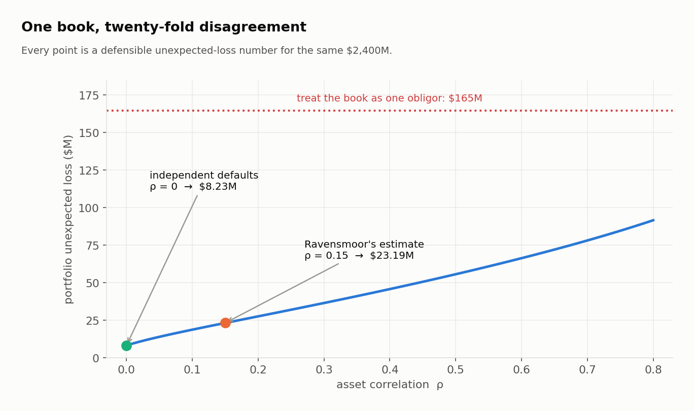
$164.61 million — which is exactly what the single-exposure formula returns if you feed it , because the formula is linear in exposure. Adding standalone unexpected losses and treating the book as one giant obligor are the same calculation. And that calculation embeds an assumption: it is only correct if every loan defaults at the same time. Standard deviations add arithmetically only under perfect positive correlation.
Route two: assume independence. If the 400 borrowers default independently, variances add rather than standard deviations, so the portfolio's unexpected loss scales with the square root of the number of loans:
$8.23 million. Twenty times smaller than route one, on the same loans.
Route three: model the correlation. Reality is neither. Borrowers are not independent — they share an economy — but they do not all fail together either. The standard approach makes each borrower's fortunes depend partly on one systematic factor and partly on its own circumstances, with an asset correlation setting the mix. At Ravensmoor's estimate of , the book's unexpected loss is $23.19 million — and, unlike the capital number below, that one can be done by hand.
The variance of a sum is the sum of every variance plus every covariance. Four hundred loans contribute 400 variances and pairwise covariances, and each covariance is the product of the two loans' loss-given-default amounts and the covariance of their default indicators:
Here is the default correlation — the correlation between two borrowers' default indicators — not the asset correlation. Turning an asset correlation of 0.15 into a default correlation needs a bivariate normal probability, which no exam calculator has, so the exam hands you . For Ravensmoor it is 0.022856 (the callout below explains why it is so much smaller than 0.15).
Worked Problem — The Book's Unexpected Loss at a Default Correlation of 0.022856
Problem. Ravensmoor's book holds 400 loans of $6 million, each with a default probability of 1.80%, an expected LGD of 45% and a standalone unexpected loss of $0.411531 million. The default correlation between any two borrowers is 0.022856. Compute the book's unexpected loss.
Solution — step by step.
- The variance terms. , and .
- One covariance. , squared 7.29. . So one pair's covariance is .
- All the pairs. pairs, contributing .
- Total. , and .
Answer: $23.19 million. Notice where it comes from: the 400 variances supply 67.74 of the 537.79, and the 159,600 covariances — each one tiny — supply the other 470.05. In a large book, the covariances are the risk.
BA II Plus keystrokes: Portfolio Unexpected Loss — n = 400; UL per loan 0.411531; EAD x LGD = 2.70; rho_D 0.022856; PD 1.80%
| Keys | Display | Note |
|---|---|---|
| 0.411531 x² × 400 = | → 67.7431 | the 400 variance terms |
| STO 1 | store them | |
| 2.7 x² × 0.022856 × 0.018 × 0.982 = | → 0.0029452 | one pair's covariance |
| × 159600 = | → 470.051 | x 400 x 399 pairs |
| + RCL 1 = √x | → 23.19 | portfolio UL, $ millions |
Expected Loss Adds. Unexpected Loss Does Not.
This is the chapter's central result, and it is worth stating as a pair:
- Expected loss is additive. $19.44 million for the book, no matter what the correlation is. Means always add.
- Unexpected loss is not additive. Between $8.23 million and $164.61 million for the same book, depending entirely on an assumption you cannot observe directly.
Every hard problem in portfolio credit risk lives in that second line. Diversification is precisely the gap between the two routes, and the size of that gap is what a correlation estimate is for.
Asset correlation is not default correlation
A trap worth pre-empting. Ravensmoor's asset correlation of 0.15 corresponds to a default correlation of only 0.0229 — the correlation between the two borrowers' default indicators. The two numbers describe the same dependence and are wildly different in magnitude, because defaults are rare events in the far tail of the asset distribution. Quoting one when a question asks for the other is a reliable way to pick a distractor.
From unexpected loss to capital
Standard deviation is a summary, not a capital requirement. To set capital, Ravensmoor simulates the whole loss distribution and reads off a high percentile. This is the one number in the chapter that cannot be done by hand: a percentile of a correlated, skewed loss distribution has no calculator formula, and the exam will always give it to you.
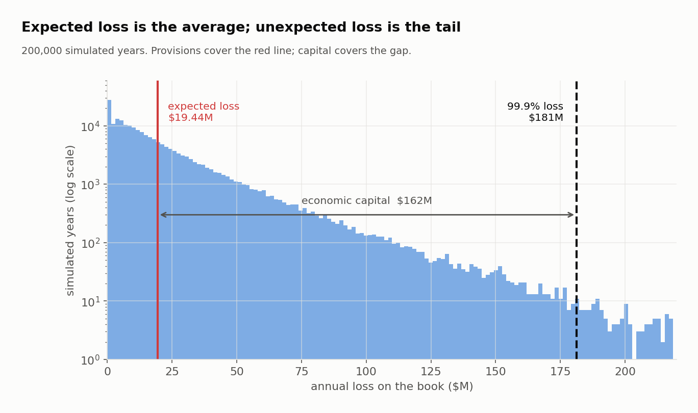
The distribution is violently asymmetric. Most years the book loses less than its average — that is what it means for a distribution with a long right tail to have a mean above its median. A few years it loses catastrophically. At the 99.9th percentile the annual loss is $181.19 million, and the distance from expected loss to that point is $161.75 million. That distance is economic capital: the cushion that lets Ravensmoor survive a one-in-a-thousand year.
Validation: the three routes and the capital number
import numpy as np
from scipy.stats import norm, multivariate_normal

n_loans, notional = 400, 6.0
pd, lgd, sigma_lgd = 0.0180, 0.45, 0.25

ul_loan = notional * np.sqrt(pd * (1 - pd) * lgd ** 2 + pd * sigma_lgd ** 2)
naive_sum = n_loans * ul_loan
independent = np.sqrt(n_loans) * ul_loan

def default_correlation(rho):
    k = norm.ppf(pd)
    joint = multivariate_normal.cdf([k, k], mean=[0, 0], cov=[[1, rho], [rho, 1]])
    return (joint - pd ** 2) / (pd * (1 - pd))

def portfolio_ul(rho):
    cov = notional ** 2 * lgd ** 2 * default_correlation(rho) * pd * (1 - pd)
    return np.sqrt(n_loans * ul_loan ** 2 + n_loans * (n_loans - 1) * cov)

print(f"route 1  perfect correlation : ${naive_sum:,.2f}M")
print(f"route 2  independent         : ${independent:,.2f}M")
print(f"route 3  rho = 0.15          : ${portfolio_ul(0.15):,.2f}M")
print(f"ratio of the extremes        : {naive_sum / independent:.0f}x")
print(f"default correlation at 0.15  : {default_correlation(0.15):.4f}")
# Output:
# route 1  perfect correlation : $164.61M
# route 2  independent         : $8.23M
# route 3  rho = 0.15          : $23.19M
# ratio of the extremes        : 20x
# default correlation at 0.15  : 0.0229
The 200,000-year simulation behind Figure 1.2 — each year draws one systematic factor, 400 borrower shocks and an LGD for every default — returns a standard deviation of $23.09 million against the formula's $23.19 million — agreement to within half a percent, which is what simulation error looks like at this sample size. When a closed form and a simulation agree to that tolerance, you have evidence that both are right; when they disagree by more, one of them has a bug.
1.6 Risk, Reward, and the Conflicts Between Them
Ravensmoor holds this book because it is paid to. The spread on the loans compensates for the 81 basis points of expected loss computed in §1.3, funds the capital held against unexpected loss, and leaves a return for shareholders. That is the risk-reward relationship in its healthy form: more risk is compensated with more expected return, and the compensation is set by the market rather than chosen by the risk taker.
The relationship breaks in a specific and predictable way: when the person taking the risk is not the person bearing it.
Three Conflicts That Bend Risk Management
Asymmetric payoffs. A loan officer paid on origination volume receives the upside of a marginal loan and none of its default losses, which arrive years later and land on the bank. Their optimal volume is higher than the bank's.
Horizon mismatch. Bonuses are annual; credit cycles are not. A strategy that earns steadily for four years and loses everything in the fifth pays four bonuses. Practitioners call this picking up nickels in front of a steamroller, and it is the structure behind several of the disasters in Chapter 7.
Information asymmetry. The desk knows its positions better than the risk function does. Where risk limits are enforced on reported numbers, the incentive is to report favourably rather than to reduce risk — which is how limit breaches become valuation disputes.
The common remedy is not exhortation. It is structural: deferred and clawback-able compensation to fix the horizon, independent valuation to fix the information asymmetry, and a risk function that reports to the board rather than to the business it monitors. Chapter 2 builds that machinery.
1.7 The Classes of Risk
Halvorsen's board report divides Ravensmoor's exposures into eight classes. The exam expects you to define each, say how it arises, and judge its impact.
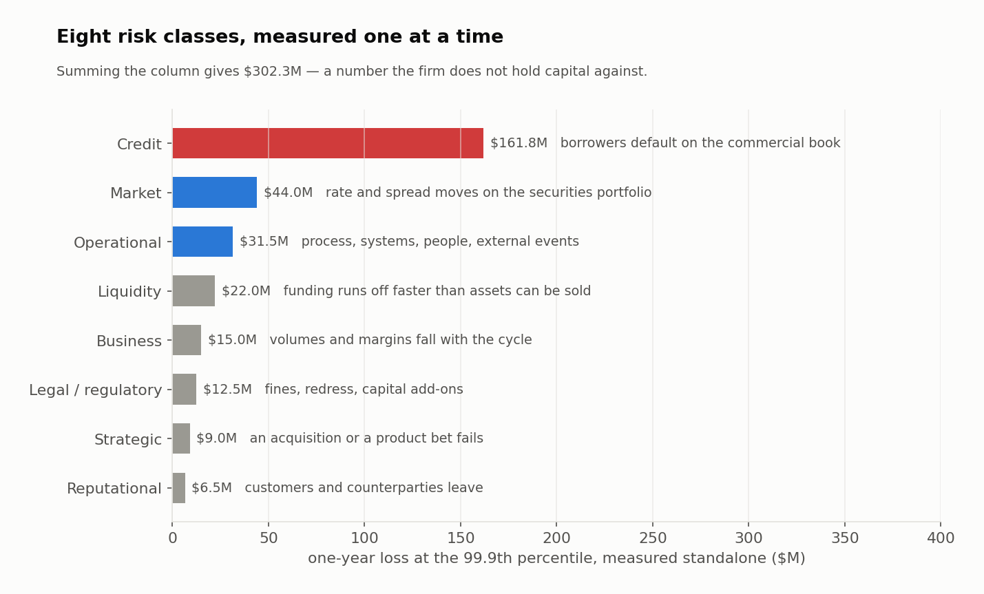
Market risk — loss from movements in market prices: interest rates, equity prices, exchange rates, commodity prices, and credit spreads. It arises wherever the firm holds a position whose value is marked to a market. Ravensmoor's securities portfolio carries $44.0 million.
Credit risk — loss from a counterparty failing to perform. It arises from lending, but equally from derivative counterparties, settlement exposure and trade receivables. At $161.8 million it is Ravensmoor's dominant exposure, which is typical for a commercial bank and the reason §1.3 to §1.5 spent so long on it.
Liquidity risk — the risk of being unable to meet obligations when due. It has two faces the exam distinguishes carefully: funding liquidity risk (the firm cannot raise cash — depositors leave, wholesale markets close) and market liquidity risk (an asset cannot be sold near its marked value). $22.0 million.
Operational risk — loss from inadequate or failed internal processes, people and systems, or from external events. Fraud, settlement failure, model error, a cyber-attack, a flood. Note that it is defined by cause, not by where the loss lands, which is why operational losses often first appear as credit or market losses. $31.5 million.
Legal and regulatory risk — loss from litigation, unenforceable contracts, regulatory penalties or changes in the rules. $12.5 million.
Business risk — loss from ordinary commercial uncertainty: volumes, margins and costs moving against the firm. It is the risk any company runs. $15.0 million.
Strategic risk — loss from major decisions that turn out badly: an acquisition that fails to integrate, a market entered at the wrong moment. Low frequency, high severity, and essentially unquantifiable in advance, which makes it a qualitative-assessment risk. $9.0 million.
Reputational risk — loss of franchise value when customers, counterparties or staff lose confidence. It is almost always a consequence of another risk crystallising rather than a primary cause. $6.5 million.
| Risk class | Arises from | 99.9th percentile loss |
|---|---|---|
| Market | positions marked to market prices, rates or spreads | $44.0M |
| Credit | a counterparty failing to perform | $161.8M |
| Liquidity | inability to raise cash or sell an asset near its marked value | $22.0M |
| Operational | failed processes, people, systems or external events | $31.5M |
| Legal and regulatory | litigation, unenforceable contracts, regulatory penalties | $12.5M |
| Business | ordinary commercial uncertainty in volumes, margins, costs | $15.0M |
| Strategic | major decisions — an acquisition, a market entered wrong | $9.0M |
| Reputational | a consequence of another risk crystallising | $6.5M |
The classification is a filing system, not a partition
Real losses refuse to sit in one box. A trader exceeds a limit and hides it: operational risk in origin, market risk in the loss, legal risk in the aftermath, reputational risk in the year following. Ravensmoor books such an event where it originated, because that is where the control belongs — but exam questions asking you to classify an event will always be answerable from the cause, so read for the cause.
1.8 Interaction and Aggregation
Figure 1.3 sums to $302.3 million. Ravensmoor does not hold $302.3 million of capital, and Halvorsen would be criticised if she asked for it. Understanding why is the last building block.
Risk factors interact. The eight classes are not eight independent machines. Consider the sequence that ended several institutions in 2008, which we will meet properly in Chapter 7:
- Credit losses rise, so the market marks down the bank's assets — credit risk becomes market risk.
- The mark-down raises doubts about solvency, so short-term lenders decline to roll their funding — market risk becomes funding liquidity risk.
- The bank sells assets to raise cash, into a market where everyone else is selling, realising losses far below model value — funding liquidity risk becomes market liquidity risk, and the losses feed back into step 1.
Each arrow is a different risk class. The whole sequence is one event. A firm that measured the three risks separately and independently would have found each survivable.
This cuts both ways, and the exam tests the direction. Interaction can make aggregate risk larger than the sum, when one risk triggers another as above. It can also make it smaller than the sum, when the risks are genuinely unrelated: a cyber-attack and a rise in credit spreads have no particular reason to arrive in the same quarter, so their 99.9th percentiles almost certainly do not coincide. Summing them assumes they do.
That is the same mathematics as §1.5, one level up. Adding the eight standalone numbers to get $302.3 million assumes perfect correlation between risk classes, exactly as adding 400 standalone unexpected losses to get $164.61 million assumed perfect correlation between borrowers.
Why Aggregation Is Hard
Four difficulties, each of which the curriculum expects you to name:
- Correlations are unobservable and unstable. They are estimated from history, and they rise in exactly the crises where the estimate matters — the phenomenon of correlations going to one.
- The measures are not commensurable. Credit risk is naturally measured over a year, market risk over a day or ten. Operational risk has no natural horizon at all. Adding numbers computed at different horizons and confidence levels is a category error before it is an arithmetic one.
- Some risks resist quantification entirely. Strategic and reputational risk have no loss distribution to combine.
- The data does not join up. The same exposure sits in several systems under several identifiers, so the firm cannot always tell whether two reported risks are two risks or one counted twice. This is the failure mode Chapter 6 is devoted to, and it is far more common than any modelling error.
1.9 Putting It All Together
Halvorsen's answer to the board, assembled from the pieces of this chapter.
The problem. How much could the $2,400 million commercial book lose in a year, and what should the bank hold against it?
Why this step: the budgeted loss. Expected loss is a recurring cost, so it is priced and provisioned, not capitalised. From §1.3: $2,400M × 1.80% × 45% = $19.44 million, an expected loss rate of 81 basis points that must appear in the loan spread.
Why this step: the variation around it. Unexpected loss is what capital absorbs. The per-loan figure from §1.4 is $0.41153 million, but the book's figure depends on correlation — and from §1.5 the honest range is $8.23 million to $164.61 million. At Ravensmoor's estimated asset correlation of 0.15, $23.19 million.
Why this step: the capital number. Standard deviation is not a capital requirement. Simulating the book gives a 99.9th-percentile annual loss of $181.19 million, so economic capital — the distance from expected loss to that percentile — is $161.75 million.
Why this step: the firm-wide view. Credit is one of eight classes. Summing all eight standalone numbers gives $302.3 million, which overstates the requirement because it assumes every tail arrives in the same year. The firm-wide number requires the aggregation judgement of §1.8, not addition.
Validation: Halvorsen's board summary, end to end
import numpy as np

n_loans, notional = 400, 6.0
pd, lgd, sigma_lgd = 0.0180, 0.45, 0.25
ead = n_loans * notional

el = ead * pd * lgd
ul_loan = notional * np.sqrt(pd * (1 - pd) * lgd ** 2 + pd * sigma_lgd ** 2)
naive_sum, independent = n_loans * ul_loan, np.sqrt(n_loans) * ul_loan
rho_d = 0.022856                     # default correlation at asset correlation 0.15
ul_015 = np.sqrt(n_loans * ul_loan ** 2
                 + n_loans * (n_loans - 1) * (notional * lgd) ** 2 * rho_d * pd * (1 - pd))
q999 = 181.19                         # INPUT: 99.9th percentile of the 200,000-year simulation

standalone_classes = [161.8, 44.0, 31.5, 22.0, 15.0, 12.5, 9.0, 6.5]

print(f"expected loss (priced, provisioned) : ${el:,.2f}M   ({pd * lgd:.2%} of exposure)")
print(f"UL, perfect correlation             : ${naive_sum:,.2f}M")
print(f"UL, independent defaults            : ${independent:,.2f}M")
print(f"UL, rho = 0.15                      : ${ul_015:,.2f}M")
print(f"99.9% loss                          : ${q999:,.2f}M")
print(f"economic capital (99.9% minus EL)   : ${q999 - el:,.2f}M")
print(f"sum of 8 standalone class numbers   : ${sum(standalone_classes):,.1f}M  <- not a capital requirement")
# Output:
# expected loss (priced, provisioned) : $19.44M   (0.81% of exposure)
# UL, perfect correlation             : $164.61M
# UL, independent defaults            : $8.23M
# UL, rho = 0.15                      : $23.19M
# 99.9% loss                          : $181.19M
# economic capital (99.9% minus EL)   : $161.75M
# sum of 8 standalone class numbers   : $302.3M  <- not a capital requirement
The board's instinct was that a bigger number is a more prudent number. The chapter's lesson is the opposite: $164.61 million and $8.23 million describe the same loans, and the difference between them is an assumption, not a margin of safety. Choosing between them is risk management. Adding up whatever numbers are to hand is not.
Chapter Summary
What You Learned in Chapter 1
- Risk is exposure to uncertainty about an outcome that matters. Risk management makes risk taking deliberate; it is not the opposite of risk taking, and a well-managed firm may hold more risk than a badly managed one.
- The toolkit is quantitative measures (for risks with history), qualitative techniques (for risks without it), and ERM as the integrating frame.
- Expected loss , or $19.44M on Ravensmoor's book — a recurring cost, priced into the spread and provisioned, never capitalised.
- Unexpected loss for a single exposure , giving $0.41153M per loan — 8.47 times its expected loss.
- EL is additive; UL is not. The book's UL is $164.61M under perfect correlation, $8.23M under independence — a twenty-fold range — and $23.19M at an asset correlation of 0.15. Adding standalone ULs and treating the book as one obligor are the same calculation.
- Economic capital is the distance from expected loss to a high percentile: $181.19M − $19.44M = $161.75M at 99.9%.
- The eight risk classes are market, credit, liquidity (funding and market), operational, legal/regulatory, business, strategic and reputational. Classify by cause, not by where the loss lands.
- Risk factors interact, so aggregate risk can exceed the sum when one risk triggers another and fall below it when risks are unrelated. Aggregation is hard because correlations are unstable, horizons differ, some risks resist quantification, and the underlying data does not join up.
What's Next
Chapter 2 takes the exposures you have just learned to name and measure and asks what Ravensmoor should do about them — accept, avoid, mitigate or transfer — and who inside the firm gets to decide. That is the pairing of risk appetite with risk governance, and it is where the $23.19 million becomes a constraint on the lending business rather than a line in a report.
The loan book itself returns in Chapter 3, where Ravensmoor sells part of it and buys protection on another part, and the expected loss you computed here turns out to be harder to move than it looks.
Concept Checks
Fast recall before the exam-format questions — no calculator needed.
-
A commercial bank decides to double its lending to a sector it understands well, after measuring the exposure, pricing the expected loss into its spreads, and confirming the position sits inside its board-approved limits. This decision is best described as:
- A failure of risk management, because the bank's measured risk has increased
- Risk avoidance, because the bank confined itself to a familiar sector
- Deliberate risk taking supported by risk management
- Risk transfer, because pricing the expected loss passes it to borrowers
-
A bank must assess the risk that a newly proposed consumer-protection statute will force it to pay customer redress. No comparable statute has previously been enacted in its jurisdiction. The most appropriate approach is:
- A qualitative assessment such as a scenario analysis or expert panel
- A parametric loss distribution calibrated to the bank's operational loss history
- An extreme value model fitted to the tail of the bank's historical losses
- Exclusion from the risk inventory until an actual loss establishes a data point
-
A portfolio of similar loans has an expected loss of $20 million. The risk manager is deciding what correlation to assume between the borrowers. Changing that assumption from independence to perfect correlation will:
- Increase both the expected loss and the unexpected loss of the portfolio
- Leave the expected loss unchanged and increase the unexpected loss
- Leave both the expected loss and the unexpected loss unchanged
- Increase the expected loss while leaving the unexpected loss unchanged
-
A risk manager computes the unexpected loss of a single loan using the standard formula, multiplies the result by the number of loans in the book, and reports the total as the portfolio's unexpected loss. This figure is:
- Correct, because unexpected loss is defined at the level of the individual exposure
- An underestimate, because it omits the covariance between the loans
- An upper bound that would only be reached if every loan defaulted together
- Correct only if the loans are of unequal size and credit quality
-
Credit losses at a bank rise, prompting the market to mark down its assets; short-term lenders then decline to roll their funding, and the bank sells assets into a falling market at prices well below model value. This sequence best illustrates:
- Operational risk, since the failure originated in the bank's internal processes
- A single risk class crystallising through several reporting lines
- Strategic risk, since the losses followed from the bank's business model
- The interaction of credit, market and liquidity risk within one event
-
A firm measures the one-year 99.9th-percentile loss for each of its eight risk classes separately and sums them. Relative to the firm's true aggregate risk at the same confidence level, the sum is most likely to be:
- Equal, because losses at a common confidence level are additive by construction
- An overstatement, because it assumes every class reaches its worst year simultaneously
- An understatement, because summing ignores the way one risk can trigger another
- Unbiased, because the overstatement from unrelated risks offsets interaction effects
-
A bank's analysts identify a possible change in commodity prices that would not affect any position the bank holds, directly or indirectly. Under the definition used in the FRM curriculum, this is:
- Not a risk to the bank, because the bank has no exposure to the outcome
- A market risk, because commodity prices are a market risk factor
- A business risk, because commodity moves affect the bank's customers
- A risk that should be recorded but assigned a probability of zero
-
A firm compares two candidate measures for the same exposure and finds that one has an unexpected loss roughly eight times its expected loss. This ratio most directly indicates that the exposure:
- Has been mismeasured, since unexpected loss cannot exceed expected loss by that margin
- Is dominated by a low-probability outcome that produces a large loss when it occurs
- Should be avoided entirely, since the variation swamps the anticipated cost
- Carries an expected loss too small to justify the cost of provisioning against it
-
A bank cannot sell a portfolio of thinly traded corporate bonds near their marked value, and separately finds that its wholesale lenders are unwilling to roll over maturing funding. These two problems are respectively:
- Funding liquidity risk and market liquidity risk
- Both instances of market risk, since both originate in market conditions
- Both instances of funding liquidity risk, since both concern access to cash
- Market liquidity risk and funding liquidity risk
-
Which of the following exposures is least suited to a quantitative risk measure and most suited to a qualitative assessment technique?
- The interest rate exposure of a portfolio of government bonds
- The credit exposure of a large pool of similar small business loans
- The settlement exposure arising from a bank's daily payment volumes
- The reputational consequence of a hypothetical failure not previously experienced
Exam-Style Practice
Standalone four-option questions at the real exam's pace — 2.4 minutes each.
Chapter 1 — The Building Blocks of Risk Management
-
A bank holds a $40 million exposure to a single borrower with a one-year default probability of 2.50%. On default the bank expects to recover 60% of the exposure. The expected loss on this exposure over one year is closest to:
- $1.00 million
- $0.40 million
- $0.60 million
- $16.00 million
-
A $25 million exposure has a one-year default probability of 4.00%, a loss given default of 50%, and a standard deviation of loss given default of 30%. The unexpected loss on this exposure is closest to:
- $0.50 million
- $4.90 million
- $2.87 million
- $2.45 million
-
A portfolio contains 100 identical loans, each with an unexpected loss of $2 million computed on a standalone basis. If the loans default independently of one another, the portfolio's unexpected loss is closest to:
- $200 million
- $20 million
- $100 million
- $2 million
-
A risk committee is told that a loan book's expected loss is $30 million and its 99.9th-percentile annual loss is $240 million. The economic capital the bank should hold against this book is closest to:
- $240 million
- $270 million
- $30 million
- $210 million
-
A trader at a bank breaches a position limit, conceals the breach by misreporting valuations, and the position is eventually closed at a large loss. Regulators later fine the bank for inadequate supervision. In the bank's risk taxonomy this event should be classified as:
- Market risk, because the loss arose from an adverse movement in market prices
- Legal and regulatory risk, because the outcome that crystallised was a fine
- Operational risk, because the event originated in failed internal processes and controls
- Strategic risk, because the bank's supervisory arrangements proved inadequate
-
Which of the following statements about aggregating risk across a financial institution is correct?
- Expected losses may be summed across risk classes, but percentile losses may not
- Both expected losses and percentile losses may be summed, provided each is measured at the same confidence level
- Neither expected losses nor percentile losses may be summed, because risk measures are never additive
- Percentile losses may be summed, but expected losses require a correlation assumption first
-
A bank's loan book has an expected loss of $50 million. A newly hired analyst argues that because the book is well diversified across 500 borrowers, the expected loss should be revised downward. The analyst's reasoning is:
- Correct, because diversification reduces the loss the bank should anticipate
- Correct, but only if the borrowers operate in genuinely unrelated industries
- Incorrect, because diversification raises expected loss by increasing the number of exposures
- Incorrect, because diversification affects the dispersion of losses rather than their mean
-
A bank estimates that it will recover 35% of exposure on a defaulted loan. The loss given default it should use in its expected loss calculation is:
- 65%
- 35%
- The recovery rate divided by one minus the default probability
- It cannot be determined without the exposure at default
-
For a single credit exposure, the variance term arising from uncertainty about the recovery rate is PD multiplied by the variance of loss given default. For a borrower with a very low default probability, this term is:
- Small in absolute terms, because it is scaled by the low default probability
- Large, because recovery uncertainty is independent of default probability
- Zero, because recovery uncertainty only matters once default is certain
- Equal to the default uncertainty term, since both are scaled by PD
-
A firm reports that its risk appetite permits an annual loss of no more than $40 million at the 95th percentile, and its measured 95th percentile loss is $38 million. On this evidence the firm's expected loss is:
- $38 million, since the percentile loss is the best estimate of the expected outcome
- $2 million, being the headroom between the measured loss and the limit
- $40 million, since the limit is set at the level of anticipated loss
- Not determinable, since a percentile of the loss distribution does not fix its mean
Get the full course: FRM Level I: Foundations of Risk Management